Overdispersion and zero-inflation

Before class starts

Download the Crabs.txt dataframe
Start a new R Script file (no Quarto for now)
Read the file and install the performance package

    crabs<-read.table("Crabs.txt",header=T)
    install.packages("performance")

Announcements

We will look at overdispersion and zero inflation
Next Week: Data wrangling (short week)
When we are back we will talk about “Generalized Mixed effects Models” –> combine mixed effects and generalized linear models
These can also have zero inflation and overdispersion
Then we will talk about GAM’s. Very important topic!
Some classes for plotting, and data management

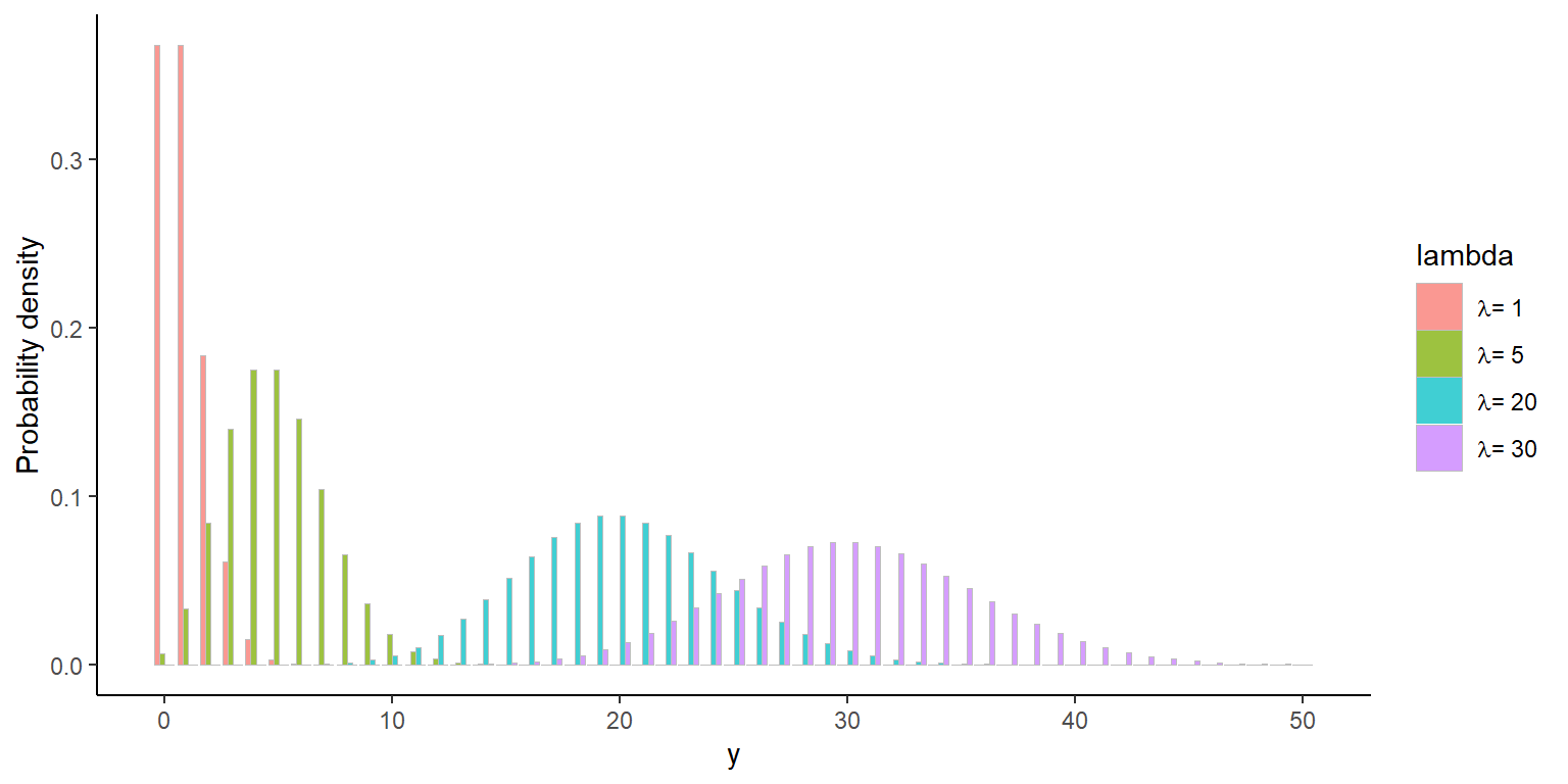
Poisson distribution

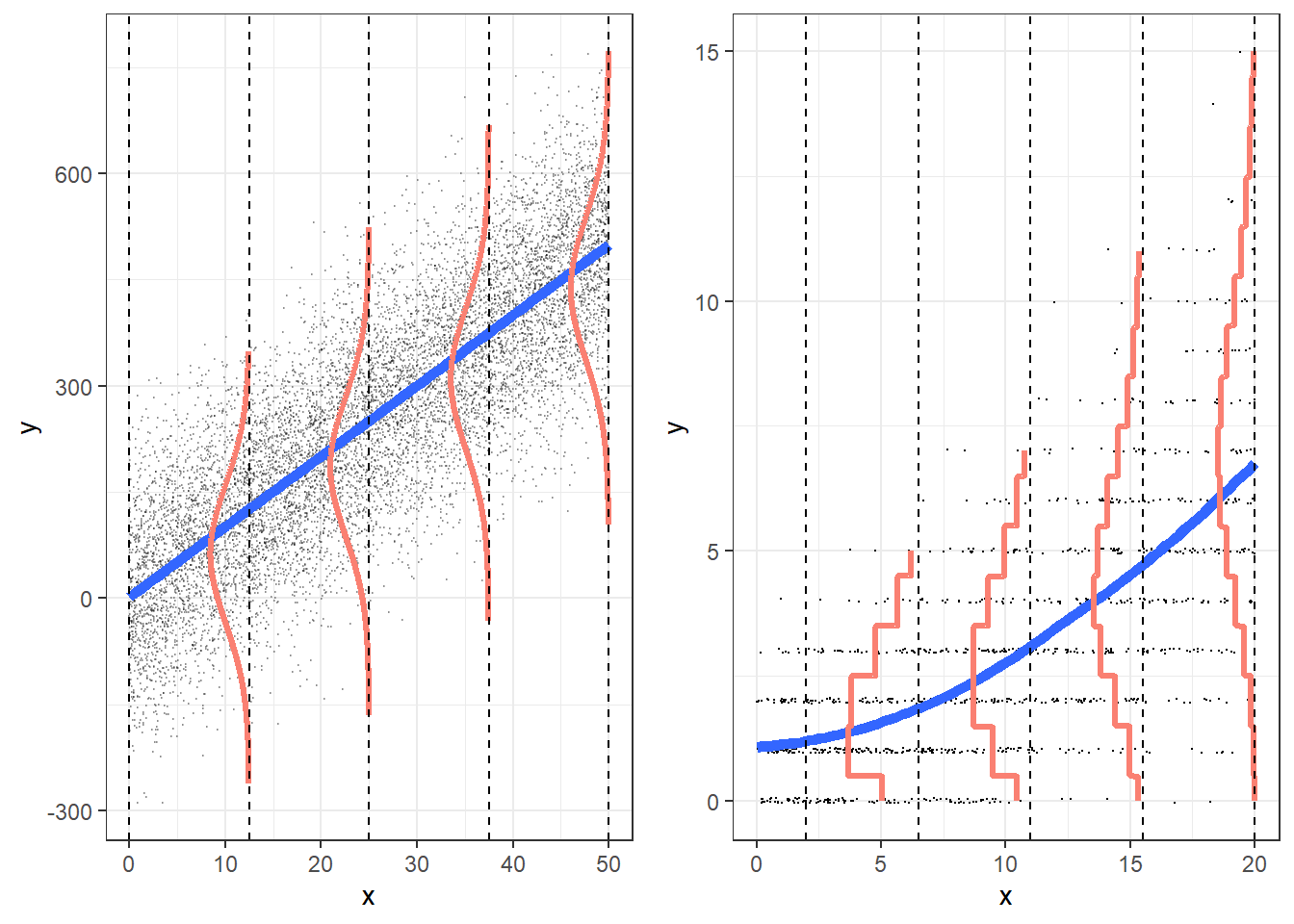
What happens when variance isn’t always \(\lambda_i\) ?

Poisson assumes that the mean \(\lambda_i\) is equal to the variance \(Var(y_i|x_i) = \lambda_i\)
This very rarely happens!
Usually \(Var(y_i|x_i) > \lambda_i\): overdispersion
We need to correct for this

Examples of overdispersion

A true Poisson distribution is completerly random!!! But if you are counting animals, are individuals randomly distributed in a field?

Fruit counts per plant (some produce a lot, some none)
Animal scat counts (animals defecate in clusters)
Pest counts in ag fields (insects tend to occur in patches)
Insurance claims

What causes overdispersion?

Omission of important variables
Measurement error
Data
NATURAL CLUSTERING!!!!
Random effects
Outliers
etc

Poisson and zeroes

Another issue with the Poisson distribution is the number of zeroes
Poisson assumes a number of zeroes given the distribution
Oftentimes we observe more zeroes than expected by the Poisson distribution
We call this zero inflation

We generally see more zeroes than predicted by \(\lambda\)

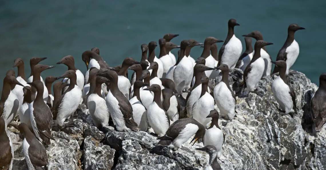
Fish catches in nets
Bird counts
Parasite counts! (example from your current assignment) – most individuals have 0! But then some have hundreds!

Reasons for zero-inflation

Structural zeroes
Imagine you are looking at the abundance of a wild vine 🍃 in the Smokies.
You set up random plots to sample using coordinates
Some areas (river and rocky shore) are unable to produce nonzero counts
You have two processes: one that produces only zeroes (inhabitable areas), and one that produces zeroes and numbers

Reasons for zero-inflation

Clustering: Can be temporal or spatial
You get many zeroes, and many high counts. High counts lead to a high \(\lambda\) which would expect low number of zeroes

Reasons for zero inflation

Observer error
For example, jaguars are very hard to observe in camera traps
If detection probability is low, then there will be lots of zeroes

Intermittent occurance

For example, number of flu infections
More zeroes in the summer than in the winter

Example

Horseshoe crabs 🦀

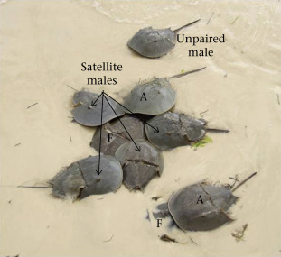
Horseshoe crabs

Females are grasped by a male for reproduction

Satellite males are individuals that do not directly grasp a female.
These males attempt to fertilize eggs externally by releasing sperm in close proximity to a nesting pair, increasing their chances of reproductive success.

Example

Horseshoe crabs 🦀

Note

Counting totality of males per female, including “attached” one

Let’s work together

crabs<-read.table("Crabs.txt",header=T)
crabs$color<-factor(crabs$color)

Example

https://users.stat.ufl.edu/

  crab sat weight width color spine
1    1   8   3.05  28.3     2     3
2    2   0   1.55  22.5     3     3
3    3   9   2.30  26.0     1     1
4    4   0   2.10  24.8     3     3
5    5   4   2.60  26.0     3     3
6    6   0   2.10  23.8     2     3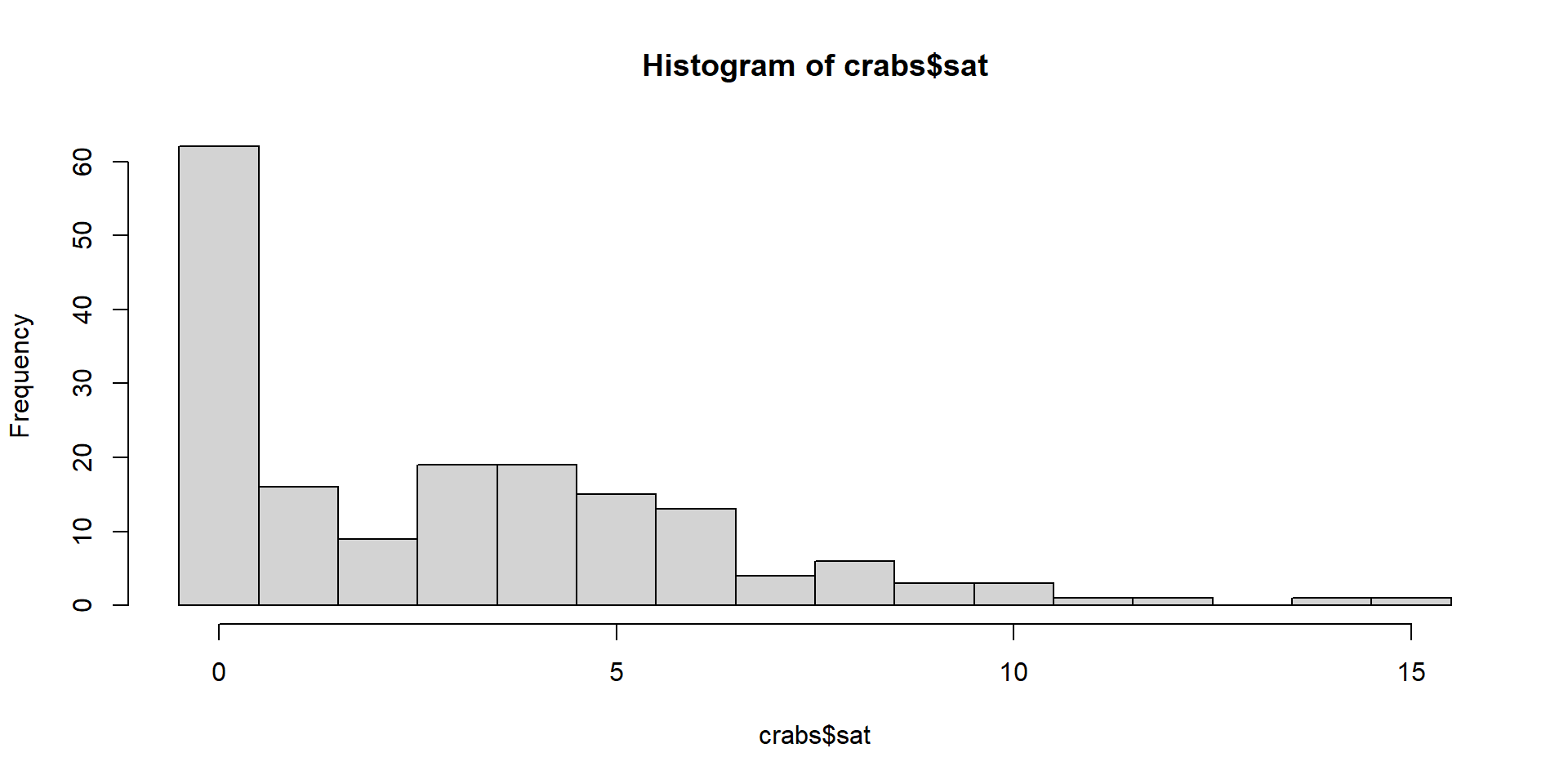

Horseshoe crabs

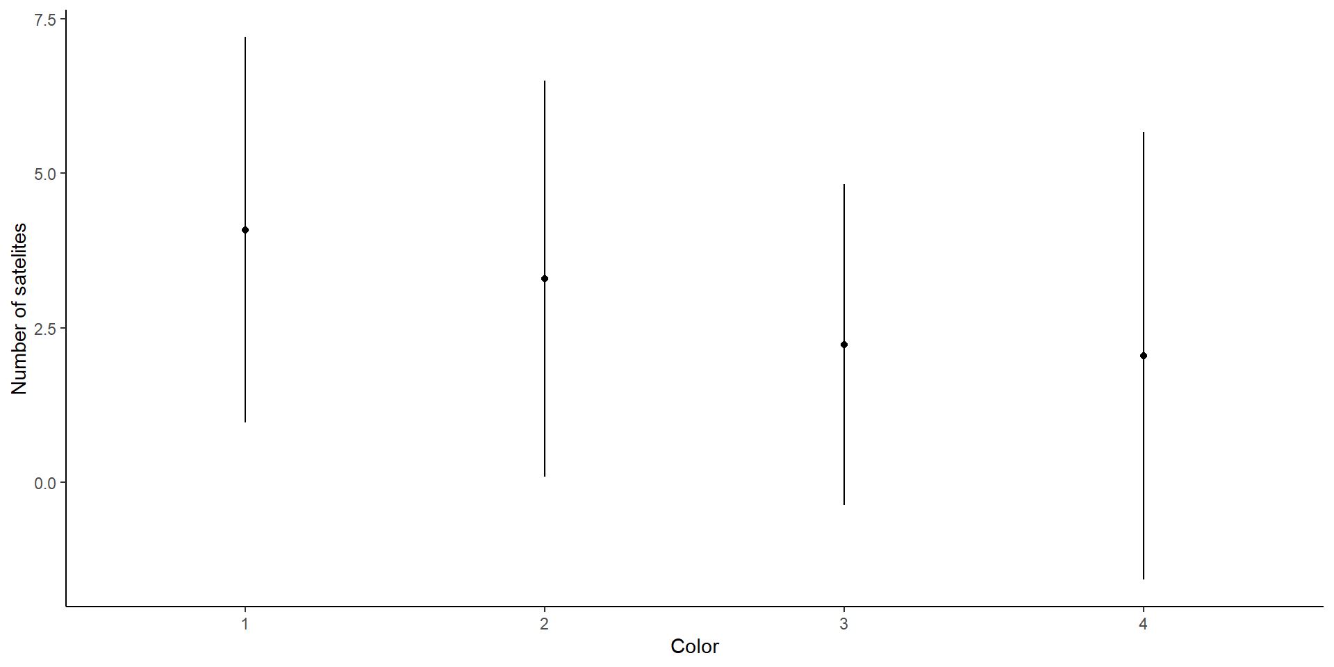
We are interested in the effects of color on the number of satellites.

First, let’s look at the model fitting:

glm1<-glm(sat~color,data=crabs,family="poisson")
summary(glm1)


Call:
glm(formula = sat ~ color, family = "poisson", data = crabs)

Coefficients:
            Estimate Std. Error z value Pr(>|z|)    
(Intercept)   1.4069     0.1429   9.848  < 2e-16 ***
color2       -0.2146     0.1536  -1.397 0.162487    
color3       -0.6061     0.1750  -3.464 0.000532 ***
color4       -0.6913     0.2065  -3.348 0.000814 ***
---
Signif. codes:  0 '***' 0.001 '**' 0.01 '*' 0.05 '.' 0.1 ' ' 1

(Dispersion parameter for poisson family taken to be 1)

    Null deviance: 632.79  on 172  degrees of freedom
Residual deviance: 609.14  on 169  degrees of freedom
AIC: 972.44

Number of Fisher Scoring iterations: 6

Looking at the data

Using performance

performance::check_overdispersion(glm1)

# Overdispersion test

       dispersion ratio =   3.454
  Pearson's Chi-Squared = 583.806
                p-value = < 0.001

What are the problems of overdispersion

Discuss, what problems can arise if there is overdispersion

Overdispersion and bias…

Overdispersion does not bias the estimates… but can affect the standard error

We can fit this in many different ways

Method 1

In Poisson:
\(\lambda_i\) is the expected value
\(\lambda_i\) is the variance
We can do a “quassipoisson”:
\(\lambda_i\) is the expected value
\(\phi\lambda_i\) is the variance
\(\phi\) is an inflation factor


Call:
glm(formula = sat ~ color, family = "quasipoisson", data = crabs)

Coefficients:
            Estimate Std. Error t value Pr(>|t|)    
(Intercept)   1.4069     0.2655   5.299  3.6e-07 ***
color2       -0.2146     0.2855  -0.751   0.4534    
color3       -0.6061     0.3252  -1.864   0.0641 .  
color4       -0.6913     0.3838  -1.801   0.0734 .  
---
Signif. codes:  0 '***' 0.001 '**' 0.01 '*' 0.05 '.' 0.1 ' ' 1

(Dispersion parameter for quasipoisson family taken to be 3.454476)

    Null deviance: 632.79  on 172  degrees of freedom
Residual deviance: 609.14  on 169  degrees of freedom
AIC: NA

Number of Fisher Scoring iterations: 6

methods


Call:
glm(formula = sat ~ color, family = "poisson", data = crabs)

Coefficients:
            Estimate Std. Error z value Pr(>|z|)    
(Intercept)   1.4069     0.1429   9.848  < 2e-16 ***
color2       -0.2146     0.1536  -1.397 0.162487    
color3       -0.6061     0.1750  -3.464 0.000532 ***
color4       -0.6913     0.2065  -3.348 0.000814 ***
---
Signif. codes:  0 '***' 0.001 '**' 0.01 '*' 0.05 '.' 0.1 ' ' 1

(Dispersion parameter for poisson family taken to be 1)

    Null deviance: 632.79  on 172  degrees of freedom
Residual deviance: 609.14  on 169  degrees of freedom
AIC: 972.44

Number of Fisher Scoring iterations: 6


Call:
glm(formula = sat ~ color, family = "quasipoisson", data = crabs)

Coefficients:
            Estimate Std. Error t value Pr(>|t|)    
(Intercept)   1.4069     0.2655   5.299  3.6e-07 ***
color2       -0.2146     0.2855  -0.751   0.4534    
color3       -0.6061     0.3252  -1.864   0.0641 .  
color4       -0.6913     0.3838  -1.801   0.0734 .  
---
Signif. codes:  0 '***' 0.001 '**' 0.01 '*' 0.05 '.' 0.1 ' ' 1

(Dispersion parameter for quasipoisson family taken to be 3.454476)

    Null deviance: 632.79  on 172  degrees of freedom
Residual deviance: 609.14  on 169  degrees of freedom
AIC: NA

Number of Fisher Scoring iterations: 6

Differences?

Analysis of Deviance Table (Type II tests)

Response: sat
      LR Chisq Df Pr(>Chisq)  
color   6.8469  3    0.07694 .
---
Signif. codes:  0 '***' 0.001 '**' 0.01 '*' 0.05 '.' 0.1 ' ' 1

qAIC

\[ QAIC = \frac{-2 * log-likelihood}{\hat{c}} + 2 * K \]

Quasipoisson has no AIC!

Back to over dispersed

performance::check_overdispersion(glm2)

# Overdispersion test

       dispersion ratio =   3.454
  Pearson's Chi-Squared = 583.806
                p-value = < 0.001

Overdispersion detected.

performance::check_zeroinflation(glm2)

# Check for zero-inflation

   Observed zeros: 62
  Predicted zeros: 11
            Ratio: 0.18

Model is underfitting zeros (probable zero-inflation).

Quasipoisson will never fix the overdispersion. The data is still overdispersed. We are just taking that into account
This is good, we are making better inferences, from imperfect data

Negative binomial distribution

Discrete probability distribution… similar to Poisson
Two parameters (like normal distribution!)
\(\mu\) and \(\theta\)
But! \(\theta\) is not variance! Remember in counts… variance increases with mean!
Variance: \(\mu + \frac{\mu^2}{\theta}\)
Think about this… what values of \(\theta\) “decrease” variance?

Negative binomial

library(MASS)
glm3<-glm.nb(sat~color,data=crabs)
summary(glm3)


Call:
glm.nb(formula = sat ~ color, data = crabs, init.theta = 0.8018786143, 
    link = log)

Coefficients:
            Estimate Std. Error z value Pr(>|z|)    
(Intercept)   1.4069     0.3526   3.990 6.61e-05 ***
color2       -0.2146     0.3750  -0.572    0.567    
color3       -0.6061     0.4036  -1.502    0.133    
color4       -0.6913     0.4508  -1.533    0.125    
---
Signif. codes:  0 '***' 0.001 '**' 0.01 '*' 0.05 '.' 0.1 ' ' 1

(Dispersion parameter for Negative Binomial(0.8019) family taken to be 1)

    Null deviance: 199.23  on 172  degrees of freedom
Residual deviance: 194.00  on 169  degrees of freedom
AIC: 772.3

Number of Fisher Scoring iterations: 1

              Theta:  0.802 
          Std. Err.:  0.136 

 2 x log-likelihood:  -762.296

Negative binomial

performance::check_overdispersion(glm3)

# Overdispersion test

       dispersion ratio =   0.793
  Pearson's Chi-Squared = 133.965
                p-value =   0.978

No overdispersion detected.

performance::check_zeroinflation(glm3)

# Check for zero-inflation

   Observed zeros: 62
  Predicted zeros: 52
            Ratio: 0.84

Model is underfitting zeros (probable zero-inflation).

Negative binomial

Usually great compromise

Closer to actual distribution

Poisson:

Analysis of Deviance Table (Type II tests)

Response: sat
      LR Chisq Df Pr(>Chisq)    
color   23.653  3  2.952e-05 ***
---
Signif. codes:  0 '***' 0.001 '**' 0.01 '*' 0.05 '.' 0.1 ' ' 1

Negative binomial:

Analysis of Deviance Table (Type II tests)

Response: sat
      LR Chisq Df Pr(>Chisq)
color   5.2285  3     0.1558

Wow! Choosing the right distribution can have a huge effect!

Hurdle models

Hurdle models combine two distributions:

“Hurdle”: Probability that the observation is 0 or not (Bernoulli)
Count data (with censored zeroes)

What distribution do we use for the count-data?
Poisson (censored)
Negative binomial (censored)

What distribution to use?

We can use both (Poisson, or negative binomial
We cannot test overdispersion or zero inflation on these models.
We can use AIC
Hurdle models are appropriate when there is a separate process that causes the zeroes…
In our example, zeroes could be governed by another cause, which is it?
Will zeroes be uniquely caused by this?

Hurdle models (poisson)

library(pscl)

Classes and Methods for R originally developed in the
Political Science Computational Laboratory
Department of Political Science
Stanford University (2002-2015),
by and under the direction of Simon Jackman.
hurdle and zeroinfl functions by Achim Zeileis.

poishurd<-hurdle(sat~color, data=crabs)
summary(poishurd)


Call:
hurdle(formula = sat ~ color, data = crabs)

Pearson residuals:
    Min      1Q  Median      3Q     Max 
-1.3218 -0.9542 -0.1097  0.6348  4.3573 

Count model coefficients (truncated poisson with log link):
            Estimate Std. Error z value Pr(>|z|)    
(Intercept)   1.6902     0.1446  11.688   <2e-16 ***
color2       -0.1894     0.1558  -1.216   0.2242    
color3       -0.3890     0.1794  -2.168   0.0302 *  
color4        0.1690     0.2083   0.811   0.4171    
Zero hurdle model coefficients (binomial with logit link):
            Estimate Std. Error z value Pr(>|z|)  
(Intercept)   1.0986     0.6667   1.648   0.0994 .
color2       -0.1226     0.7053  -0.174   0.8620  
color3       -0.7309     0.7338  -0.996   0.3192  
color4       -1.8608     0.8087  -2.301   0.0214 *
---
Signif. codes:  0 '***' 0.001 '**' 0.01 '*' 0.05 '.' 0.1 ' ' 1 

Number of iterations in BFGS optimization: 11 
Log-likelihood: -369.5 on 8 Df

Hurdle models (neg binomial)

nbhurd<-hurdle(sat~color, data=crabs, dist="negbin")
summary(nbhurd)


Call:
hurdle(formula = sat ~ color, data = crabs, dist = "negbin")

Pearson residuals:
     Min       1Q   Median       3Q      Max 
-1.12222 -0.86733 -0.09559  0.55308  3.79647 

Count model coefficients (truncated negbin with log link):
            Estimate Std. Error z value Pr(>|z|)    
(Intercept)   1.6684     0.2109   7.910 2.57e-15 ***
color2       -0.1998     0.2257  -0.885    0.376    
color3       -0.4124     0.2543  -1.622    0.105    
color4        0.1763     0.3100   0.569    0.570    
Log(theta)    1.6463     0.3696   4.454 8.43e-06 ***
Zero hurdle model coefficients (binomial with logit link):
            Estimate Std. Error z value Pr(>|z|)  
(Intercept)   1.0986     0.6667   1.648   0.0994 .
color2       -0.1226     0.7053  -0.174   0.8620  
color3       -0.7309     0.7338  -0.996   0.3192  
color4       -1.8608     0.8087  -2.301   0.0214 *
---
Signif. codes:  0 '***' 0.001 '**' 0.01 '*' 0.05 '.' 0.1 ' ' 1 

Theta: count = 5.1879
Number of iterations in BFGS optimization: 20 
Log-likelihood: -359.6 on 9 Df

IMPORTANT! Hurdle models

Hurdle models can use different covariates for each submodel!

What does this mean?
What could we use here?

Zero inflated mixture models

If zeroes are not uniquely caused by an independent event, then zero inflated mixture models are the way to go.

Maybe some crabs that could breed, won’t…
Two types of zeroes: structural and sampling (Hurdle models only take into account structural zeroes)
Zero inflated mixture models can be used in this case
Poisson or Negative binomial

zeroinfl1<-zeroinfl(sat~color|.,data=crabs)
summary(zeroinfl1)


Call:
zeroinfl(formula = sat ~ color | ., data = crabs)

Pearson residuals:
    Min      1Q  Median      3Q     Max 
-1.7392 -0.7983 -0.3146  0.6155  4.5387 

Count model coefficients (poisson with log link):
            Estimate Std. Error z value Pr(>|z|)    
(Intercept)   1.6897     0.1448  11.670   <2e-16 ***
color2       -0.1889     0.1560  -1.211   0.2259    
color3       -0.3793     0.1784  -2.126   0.0335 *  
color4        0.1692     0.2084   0.812   0.4169    

Zero-inflation model coefficients (binomial with logit link):
              Estimate Std. Error z value Pr(>|z|)  
(Intercept)  8.8735573  3.8819151   2.286   0.0223 *
crab        -0.0004505  0.0037863  -0.119   0.9053  
weight      -0.8315211  0.7196025  -1.156   0.2479  
width       -0.2815991  0.1957250  -1.439   0.1502  
color2       0.0674027  0.8005044   0.084   0.9329  
color3       0.4444279  0.8687349   0.512   0.6089  
color4       1.5955897  0.9455045   1.688   0.0915 .
spine       -0.2234416  0.2564196  -0.871   0.3835  
---
Signif. codes:  0 '***' 0.001 '**' 0.01 '*' 0.05 '.' 0.1 ' ' 1 

Number of iterations in BFGS optimization: 22 
Log-likelihood: -356.4 on 12 Df

library(pscl)
zeroinfl2<-zeroinfl(sat~color|.,data=crabs, dist="negbin")
summary(zeroinfl2)


Call:
zeroinfl(formula = sat ~ color | ., data = crabs, dist = "negbin")

Pearson residuals:
    Min      1Q  Median      3Q     Max 
-1.4036 -0.7258 -0.2650  0.5328  3.7532 

Count model coefficients (negbin with log link):
            Estimate Std. Error z value Pr(>|z|)    
(Intercept)   1.6671     0.2083   8.005 1.19e-15 ***
color2       -0.1947     0.2226  -0.875    0.382    
color3       -0.3817     0.2487  -1.535    0.125    
color4        0.1769     0.3056   0.579    0.563    
Log(theta)    1.7103     0.3643   4.695 2.67e-06 ***

Zero-inflation model coefficients (binomial with logit link):
              Estimate Std. Error z value Pr(>|z|)  
(Intercept)  9.0946460  4.0865995   2.225   0.0260 *
crab        -0.0006212  0.0040847  -0.152   0.8791  
weight      -0.9176722  0.7669885  -1.196   0.2315  
width       -0.2843510  0.2056865  -1.382   0.1668  
color2       0.0371842  0.8735382   0.043   0.9660  
color3       0.4690976  0.9405064   0.499   0.6179  
color4       1.6792645  1.0120373   1.659   0.0971 .
spine       -0.2411114  0.2773722  -0.869   0.3847  
---
Signif. codes:  0 '***' 0.001 '**' 0.01 '*' 0.05 '.' 0.1 ' ' 1 

Theta = 5.5304 
Number of iterations in BFGS optimization: 26 
Log-likelihood: -346.9 on 13 Df

Model comparisons


Model selection based on AICc:

            K   AICc Delta_AICc AICcWt Cum.Wt      LL
zeronb     13 722.15       0.00      1      1 -346.93
nbhurdle    9 738.39      16.24      1      1 -359.64
zeropois   12 738.79      16.64      0      1 -356.42
poishurdle  8 755.93      33.78      0      1 -369.53
neg.bin     5 772.66      50.51      1      1 -381.15
Poissonglm  4 972.67     250.53      1      1 -482.22

Overdispersion and zero-inflation

Before class starts

Announcements

Poisson distribution

Poisson distribution

What happens when variance isn’t always \(\lambda_i\) ?

Examples of overdispersion

What causes overdispersion?

Poisson and zeroes

We generally see more zeroes than predicted by \(\lambda\)

Reasons for zero-inflation

Reasons for zero-inflation

Reasons for zero inflation

Intermittent occurance

Example

Horseshoe crabs

Example

Note

Let’s work together

Example

Horseshoe crabs

Looking at the data

Using performance

What are the problems of overdispersion

Overdispersion and bias…

Method 1

methods

qAIC

Back to over dispersed

Other solutions

Negative binomial distribution

Negative binomial

Negative binomial

Negative binomial

Hurdle models

What distribution to use?

Hurdle models (poisson)

Hurdle models (neg binomial)

IMPORTANT! Hurdle models

Zero inflated mixture models

Model comparisons