Announcements
Mixed Effects Models this week (lab) –> One “lab” with me
Next week: Generalized Mixed Effects Models (No Lab)
Next week (Friday): Work on your plot
Back to our example
Back to our example
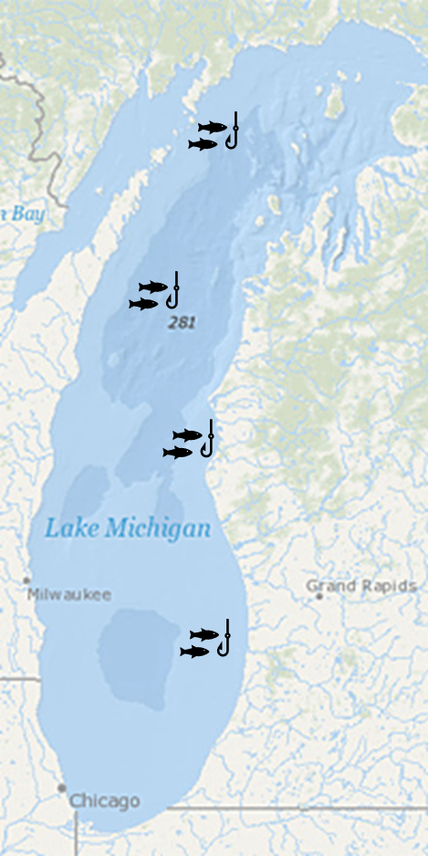
We set 4 nets
Sites were randomly chosen
We are interested in the content of Hg in Walleye
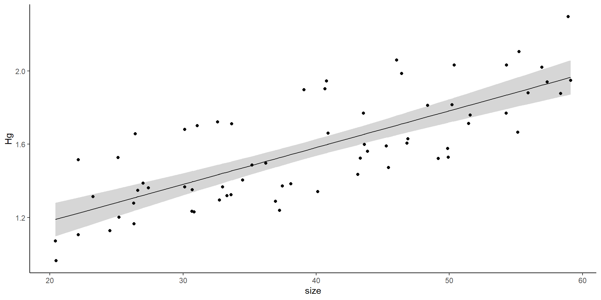
Hg is correlated with size. The bigger the fish, the higher Hg content it has
So, normally we could do one thing:
\(E[Hg_i] = \beta_0 + \beta_1 \times size_{i}\)
\(y_i \sim N(mean = E[Hg_i], \sigma)\)
Linear model
Linear model
Call:
lm(formula = Hg ~ size, data = HgDat_df)

Residuals:
     Min       1Q   Median       3Q      Max
-0.28712 -0.13507 -0.05476  0.10644  0.35471

Coefficients:
            Estimate Std. Error t value Pr(>|t|)
(Intercept) 0.781644   0.084717   9.227 1.98e-13 ***
size        0.020017   0.002067   9.682 3.16e-14 ***
---
Signif. codes:  0 '***' 0.001 '**' 0.01 '*' 0.05 '.' 0.1 ' ' 1

Residual standard error: 0.1874 on 65 degrees of freedom
Multiple R-squared:  0.5905,    Adjusted R-squared:  0.5843
F-statistic: 93.75 on 1 and 65 DF,  p-value: 3.165e-14
Assumptions of a Linear Model
Normality
Homoschedasticity
Linearity
Independence –> of data
Independence –> of error (or residuals)
Linear Model
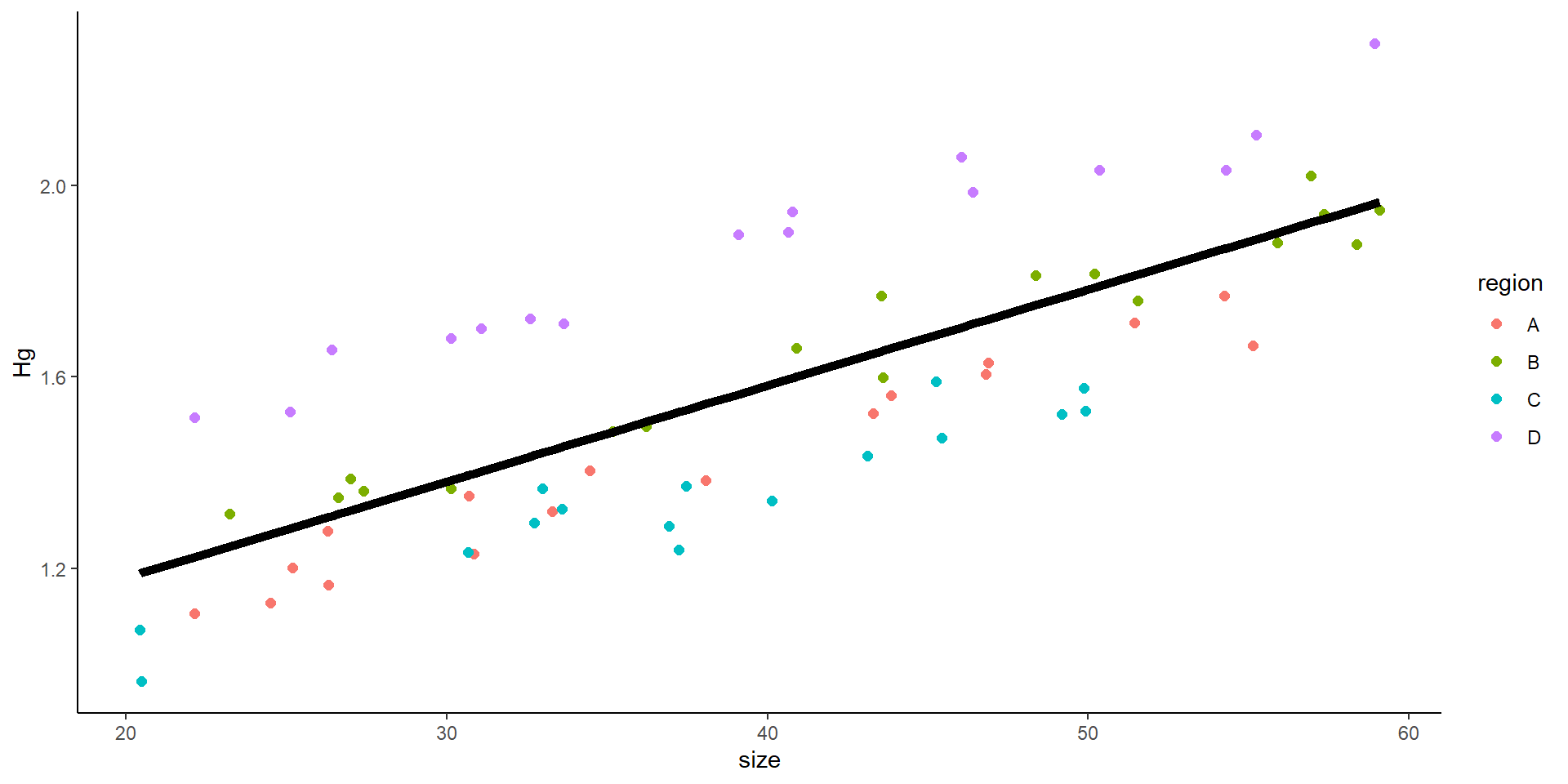
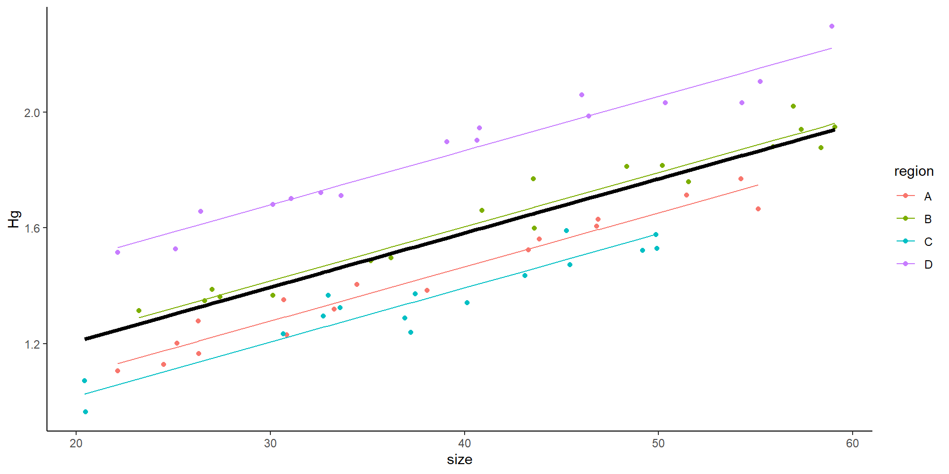
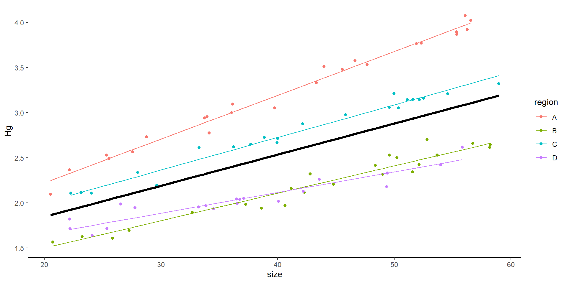
If we plot the “sites”?
The variance can affect the slope, the intercept, or both
Mixed model
No mixed model:
\[
Hg_i \sim \beta_0 + \beta_1size_{i} + \epsilon_i
\]
What is i?
We have two sources of variance (error): The fish (i) and the net (j)
i individuals, j sites (4)
Mixed model
No mixed model:
\[Hg_i \sim \beta_0 + \beta_1size_{i} + \epsilon_i
\]
Mixed model: i individuals and j sites introduced as error.
We can do a mixed model with mixed intercept or mixed slope
mixed intercept (nets only affect the intercept) –> analogous to additive model:
\[
Hg_{ij} \sim \underbrace{(\beta_0 +\underbrace{\gamma_j}_{\text{Random intercept}})}_{intercept} + \underbrace{\beta_1size_{i}}_{slope} +\underbrace{\epsilon_i}_\text{ind var}
\]
Variance comes from random “selection” of fish within a net
\(\epsilon_i \sim N(0, \sigma)\)
Variance comes from random “selection” of sites
\(\gamma_j \sim N(0,\sigma_j)\)
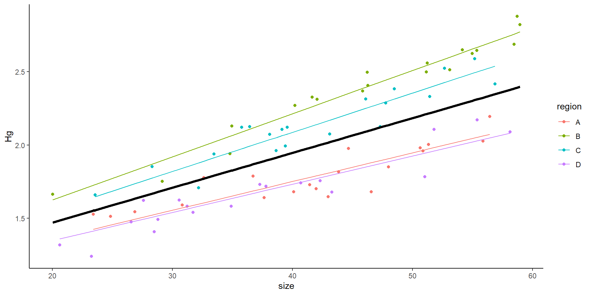
What does a mixed intercept mean?
Mixed model with random intercept
This is the result of a mixed model:
What does the random intercept mean?
Why not simply do:
\(Hg_i \sim \beta_0 + \beta_1size_{i} + \beta_2rB_{i} + \beta_3rC_{i} + \beta_4rD_{i}+ \epsilon_i\) Model with effect of site
Mixed model with random intercept
Really show that how far each point is from the mean depends on two things: Variance of site and variance of points.
Show that the fixed effects would really just predict the main line, then, the actual observations are because of that variance
 Family: gaussian  ( identity )
Formula:          Hg ~ size + (1 | region)
Data: HgDat_df

     AIC      BIC   logLik deviance df.resid
  -177.1   -168.3     92.6   -185.1       63

Random effects:

Conditional model:
 Groups   Name        Variance Std.Dev.
 region   (Intercept) 0.032847 0.18124
 Residual             0.002688 0.05184
Number of obs: 67, groups:  region, 4

Dispersion estimate for gaussian family (sigma^2): 0.00269

Conditional model:
             Estimate Std. Error z value Pr(>|z|)
(Intercept) 0.8357038  0.0937058    8.92   <2e-16 ***
size        0.0186742  0.0005839   31.98   <2e-16 ***
---
Signif. codes:  0 '***' 0.001 '**' 0.01 '*' 0.05 '.' 0.1 ' ' 1
\[
Hg_{ij} = \underbrace{(\beta_0 +\underbrace{\gamma_j}_{\text{Random intercept}})}_{intercept} + \underbrace{\beta_1size_{i}}_{slope} +\underbrace{\epsilon_i}_\text{ind var}
\]
Where:
\[
\epsilon_i \sim N(0,\sigma^2)
\]
\[
\gamma_j \sim N(0,\sigma^2_\gamma)
\]
Mixed effects models: how to run them?
library (glmmTMB)<- glmmTMB (Hg~ size + (1 | region), data= HgDat_df)
Random effects are specified as \(x|g\)
x is an effect
g is grouping factor (categorical)
\(1|region\)
Effect -> 1 (intercept)
Mixed effects model output
 Family: gaussian  ( identity )
Formula:          Hg ~ size + (1 | region)
Data: HgDat_df

     AIC      BIC   logLik deviance df.resid
  -177.1   -168.3     92.6   -185.1       63

Random effects:

Conditional model:
 Groups   Name        Variance Std.Dev.
 region   (Intercept) 0.032847 0.18124
 Residual             0.002688 0.05184
Number of obs: 67, groups:  region, 4

Dispersion estimate for gaussian family (sigma^2): 0.00269

Conditional model:
             Estimate Std. Error z value Pr(>|z|)
(Intercept) 0.8357038  0.0937058    8.92   <2e-16 ***
size        0.0186742  0.0005839   31.98   <2e-16 ***
---
Signif. codes:  0 '***' 0.001 '**' 0.01 '*' 0.05 '.' 0.1 ' ' 1
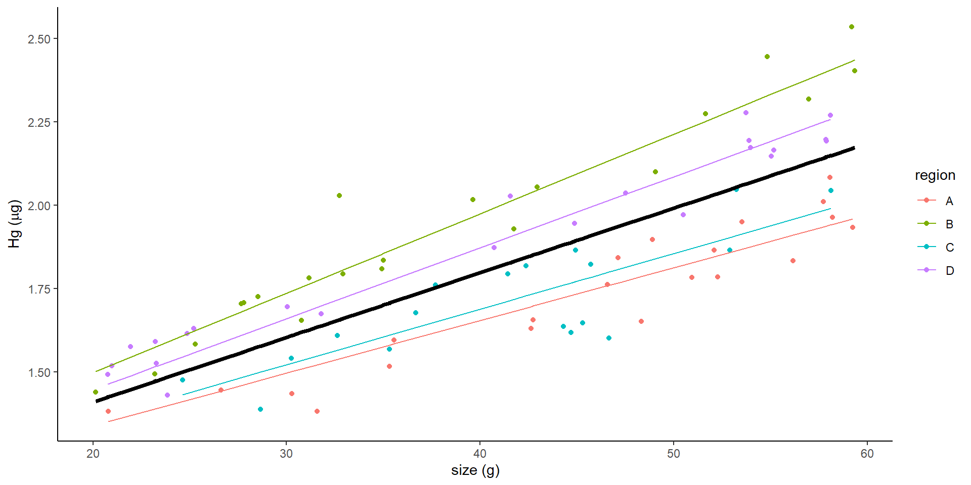
Mixed model with random intercept and random slope
\[ Hg_i \sim \beta_0 + \beta_1size_{i} + \epsilon_i \]
i individuals, j sites (4)
\[ Hg_{ij} \sim \underbrace{(\beta_0 +\underbrace{\gamma_j}_{\text{Random intercept}})}_{intercept} + \underbrace{(\beta_1+\underbrace{\psi_j}_{\text{Random slope}})size_{i}}_{slope} +\underbrace{\epsilon_i}_\text{ind var} \]
Variance comes from random “selection” of fish within a net
Variance comes from random “selection” of sites
Where,
\[
\epsilon_i \sim N(0,\sigma^2)
\]
\[
\gamma_j \sim N(0,\sigma^2_\gamma)
\]
\[
\psi_j \sim N(0,\sigma^2_\psi)
\]
Random slope and intercept
<- glmmTMB (Hg~ size + (1 + size| region), data= HgDat2_df)summary (m3)
 Family: gaussian  ( identity )
Formula:          Hg ~ size + (1 + size | region)
Data: HgDat2_df

     AIC      BIC   logLik deviance df.resid
  -153.4   -138.4     82.7   -165.4       83

Random effects:

Conditional model:
 Groups   Name        Variance  Std.Dev. Corr
 region   (Intercept) 2.765e-02 0.166290
          size        8.865e-05 0.009415 0.30
 Residual             6.287e-03 0.079291
Number of obs: 89, groups:  region, 4

Dispersion estimate for gaussian family (sigma^2): 0.00629

Conditional model:
            Estimate Std. Error z value Pr(>|z|)
(Intercept) 1.157873   0.089296  12.967  < 2e-16 ***
size        0.034451   0.004772   7.219 5.23e-13 ***
---
Signif. codes:  0 '***' 0.001 '**' 0.01 '*' 0.05 '.' 0.1 ' ' 1
Random effects are specified as \(x|g\)
x is an effect
g is grouping factor (categorical)
\(1 + size|region\)
Effect -> 1 (intercept) + size
Random slope and intercept
Only random slope
 Family: gaussian  ( identity )
Formula:          Hg ~ size + (0 + size | region)
Data: HgDat2_df

     AIC      BIC   logLik deviance df.resid
  -158.4   -148.8     83.2   -166.4       79

Random effects:

Conditional model:
 Groups   Name Variance  Std.Dev.
 region   size 1.103e-05 0.003321
 Residual      6.441e-03 0.080256
Number of obs: 83, groups:  region, 4

Dispersion estimate for gaussian family (sigma^2): 0.00644

Conditional model:
            Estimate Std. Error z value Pr(>|z|)
(Intercept) 1.021430   0.031578   32.35   <2e-16 ***
size        0.019400   0.001817   10.68   <2e-16 ***
---
Signif. codes:  0 '***' 0.001 '**' 0.01 '*' 0.05 '.' 0.1 ' ' 1
We don’t do this
\(E(Hg_i) = \beta_0 + \beta_1*size_{i}\)
Pseudoreplication
\(E(Hg_i) = \beta_0 + \beta_1size_{i} + \beta_2 site2_i + \beta_3 site3_i + \beta_4 site4_i\)
We don’t care about the specific sites… we want whole population-wide!
What do we want to know?
Mercury concentration population-wide
Variance introduces by placement of the nets
\[ Hg_{ij} \sim \underbrace{(\beta_0 +\underbrace{\gamma_j}_{\text{Random intercept}})}_{intercept} + \underbrace{(\beta_1+\underbrace{\psi_j}_{\text{Random slope}})size_{i}}_{slope} +\underbrace{\epsilon}_\text{ind var} \]
\(\gamma_j \sim Normal(0,\sigma_\gamma)\)
\(\psi_j \sim Normal(0,\sigma_\psi)\)
\(\epsilon \sim Normal(0,\sigma)\)
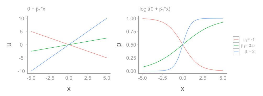
GLM’s
How many assumptions does it break?
GLM’s
GLM’s
GLM’s
Mixed models
If we set all random effects to zero, we get population mean, and predicted value for a random individual
Mixed effects
Set nets on each of those sites
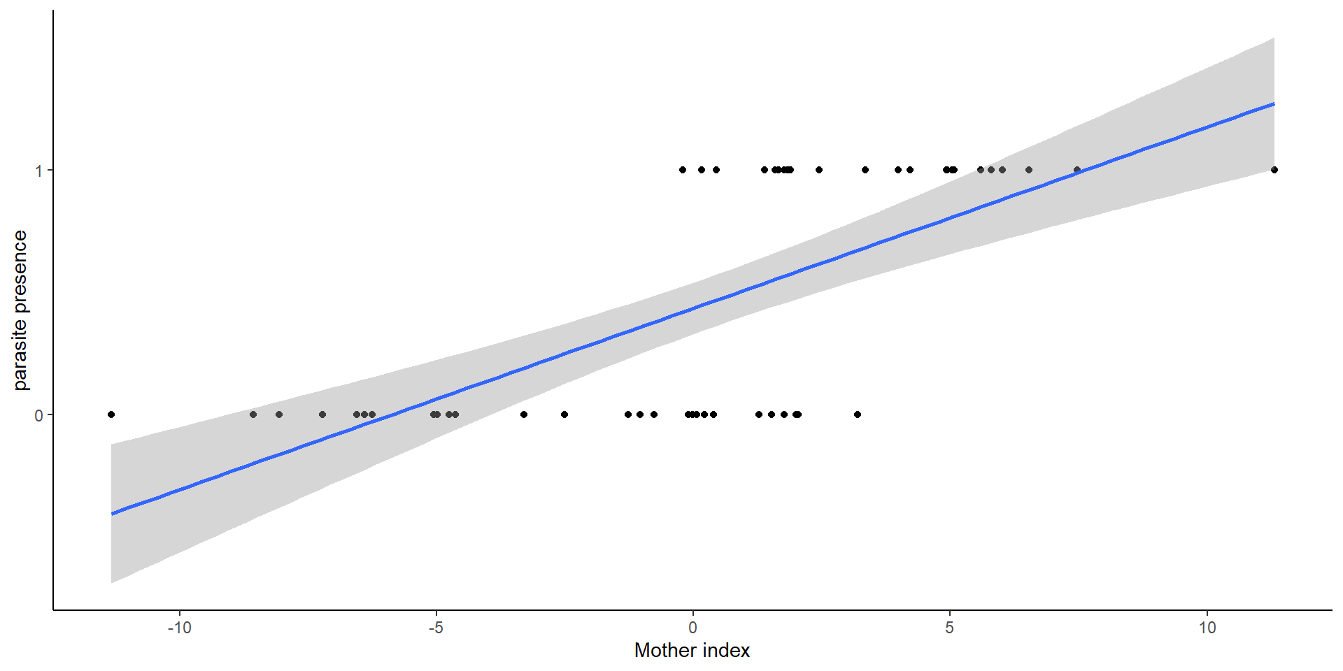
Measure 50, 43, 67, and 90 fish. For number of parasites OR presence of parasites?
Generalized linear mixed effects models
GLMM’s
How can we run mixed effects models?
Easy way: Add random effects to the linear predictor, leading to generalized linear mixed effect models
Essentially, you have two sources of variation
One is normally dsitributed, the other one is distributed according to a different distribution
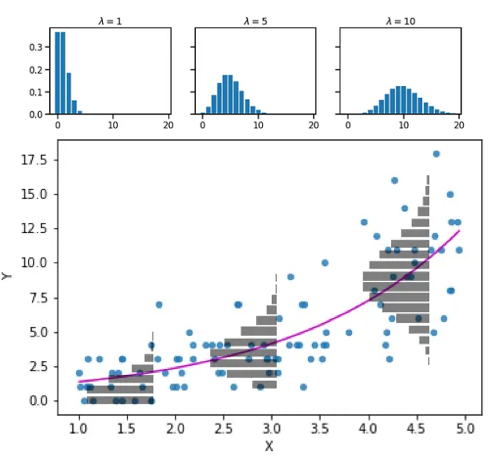
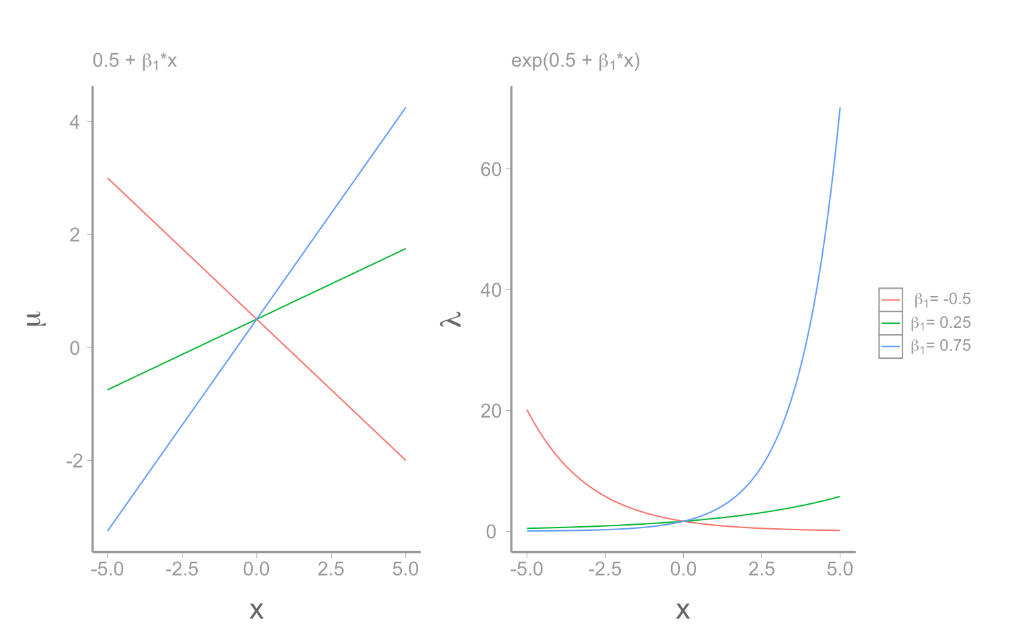
Example
A poisson glm:
\(log(\lambda) = \beta_0 + \beta_1x_i\)
\(y_i \sim Poisson(\lambda)\)
A glmm: Poisson-normal
\(log(\lambda) = (\beta_0+\gamma) + (\beta_1+\psi)x_{ij}\)
\(\gamma \sim N(0,\sigma_\gamma)\) , \(\psi\sim N(0,\sigma_\psi)\)
\(y_i \sim Poisson(\lambda)\)
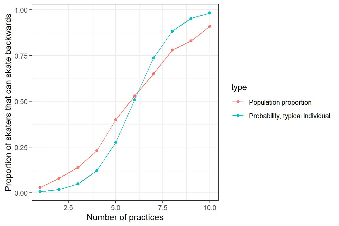
Parameter interpretation
Not easy to interpret!
In random effects if we set all random effects to 0, then we estimate the mean for a “typical” individual
“typical means subject, site, individual, etc.”
The variances are in different distributions
Typical individual does not equal “population average response”
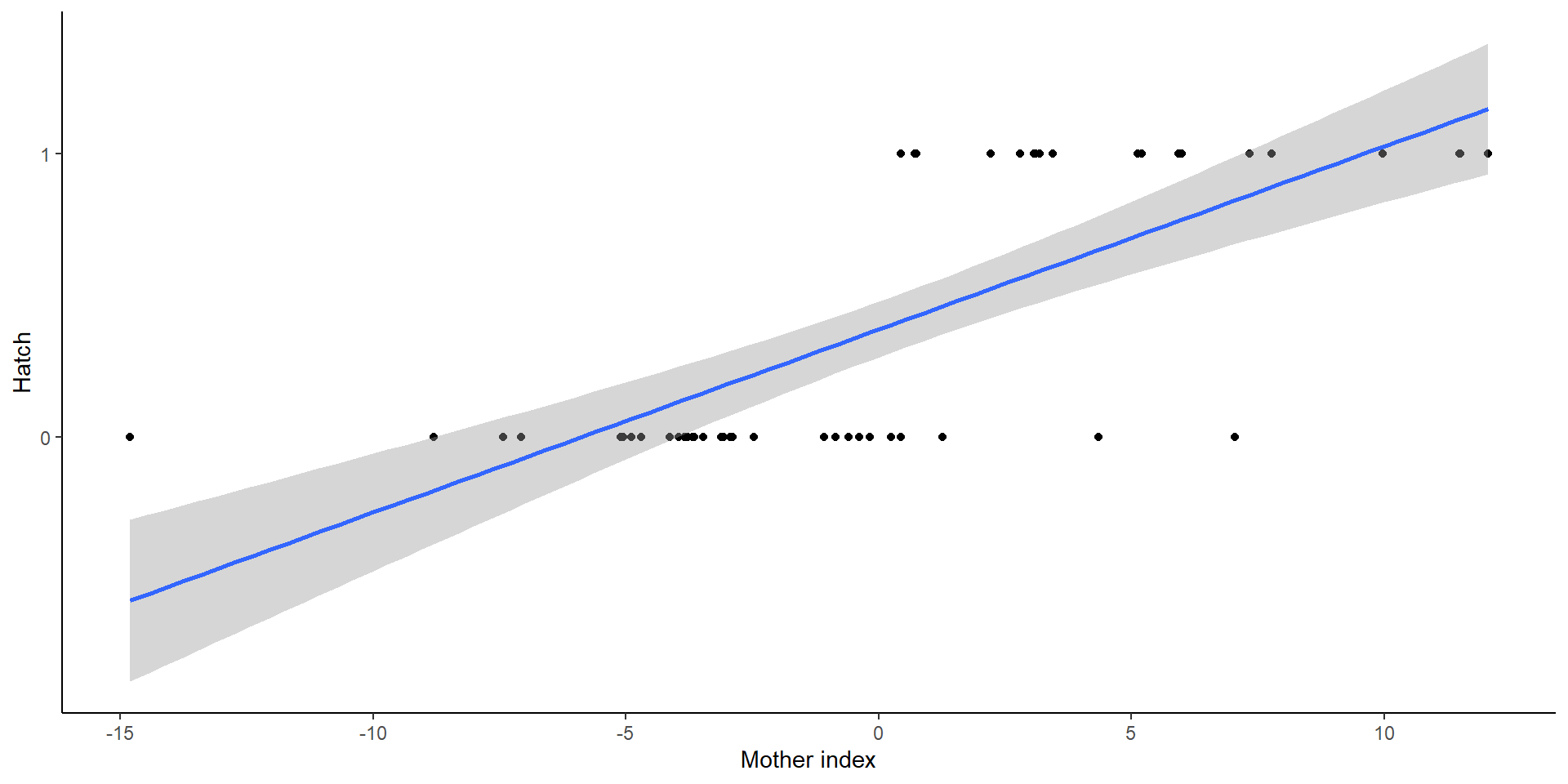
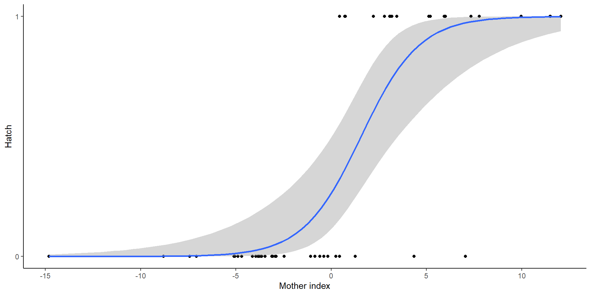
Example
Both curves are not lining up
Due to non-logit transformations (random effects are normal)
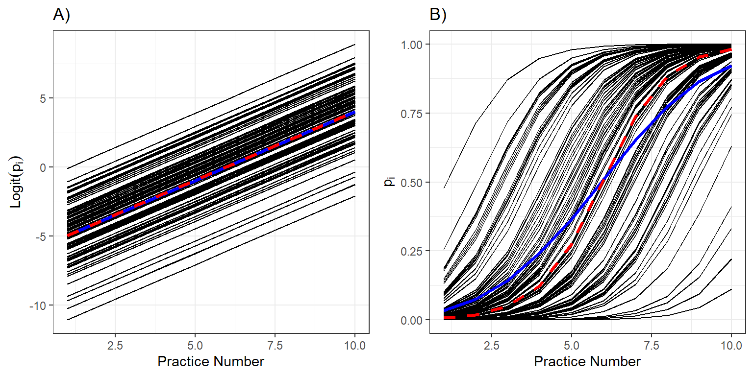
Interpreting data
Individual response curves (black), the response curve for a typical individual with random effects at zeroes, and the population mean response curve (blue) and on the logit and probability scales
In other words
A glmm: Poisson-normal
\(log(\lambda) = (\beta_0+\gamma) + (\beta_1+\psi)x_{ij}\)
\(\gamma \sim N(0,\sigma_\gamma)\) , \(\psi\sim N(0,\sigma_\psi)\)
\(y_i \sim Poisson(\lambda)\)
Because of non linearity if we set \(\gamma\) and \(\psi\) to 0’s, the end result will be different than if we get the mean of the overall response
Take away
If you do glmm’s be very careful about interpretation
In general, transforming data can be risky
Solutions?
Package GLMMadaptive estimates marginal means
How can we run mixed effects models?
Easy way: Add random effects to the linear predictor, leading to generalized linear mixed effect models
Hard way: Generalized Estimating Equations
https://fw8051statistics4ecologists.netlify.app/gee
RIKZ data
RIKZ data
RIKZ institute
Inter-tidal area (AKA beach): 9
In each beach, 5 samples were taken
Response variable: macro-fauna richness (AKA number of species)
NAP: height of sampling station compared to mean tidal level
Exposure (index). Of multiple environmental conditions. Treated as categorical, as there are three levels
RIKZ data
flowchart TD

  A[RIKZ DATA] --> B(Beach 1)
  A --> C(Beach 2)
  A --> E(Beach 9)
  B --> F(site 1)
  B --> G(site 2)
  B --> H(site 3)
  B --> I(site 4)
  B --> J(site 5)
  C --> K(site 1)
  C --> L(site 2)
  C --> M(site 3)
  C --> N(site 4)
  C --> O(site 5)
  E --> P(site 1)
  E --> Q(site 2)
  E --> R(site 3)
  E --> S(site 4)
  E --> T(site 5)
Let’s work on this example
Objective
flowchart TD

  A[RIKZ DATA] --> B(Beach 1)
  A --> C(Beach 2)
  A --> E(Beach 9)
  B --> F(site 1)
  B --> G(site 2)
  B --> H(site 3)
  B --> I(site 4)
  B --> J(site 5)
  C --> K(site 1)
  C --> L(site 2)
  C --> M(site 3)
  C --> N(site 4)
  C --> O(site 5)
  E --> P(site 1)
  E --> Q(site 2)
  E --> R(site 3)
  E --> S(site 4)
  E --> T(site 5)
Exploring whether there is a relationship between richness and the two factors: NAP and exposure
We have an N of 45… but do we?
We have multiple potential alternatives: there is an effect of NAP, an effect of Exposure, an effect of both, of neither
Also… there are mixed effects
Random intercept, random slope, both? –> let’s wait to discuss this
Step 1: Read the data… there is a potential issue
<- read.table (file = "RIKZ.txt" , header = TRUE , dec = "," )str (rikz)
Step 2: decide our analysis! 🤔 Any ideas? any details?
rikz<-read.table(file = “RIKZ.txt”, header = TRUE, dec = “,”)
rikz$NAP<-as.numeric(rikz$NAP)
rikz$Beach<-factor(rikz$Beach)
rikz$Exposure<-factor(rikz$Exposure)
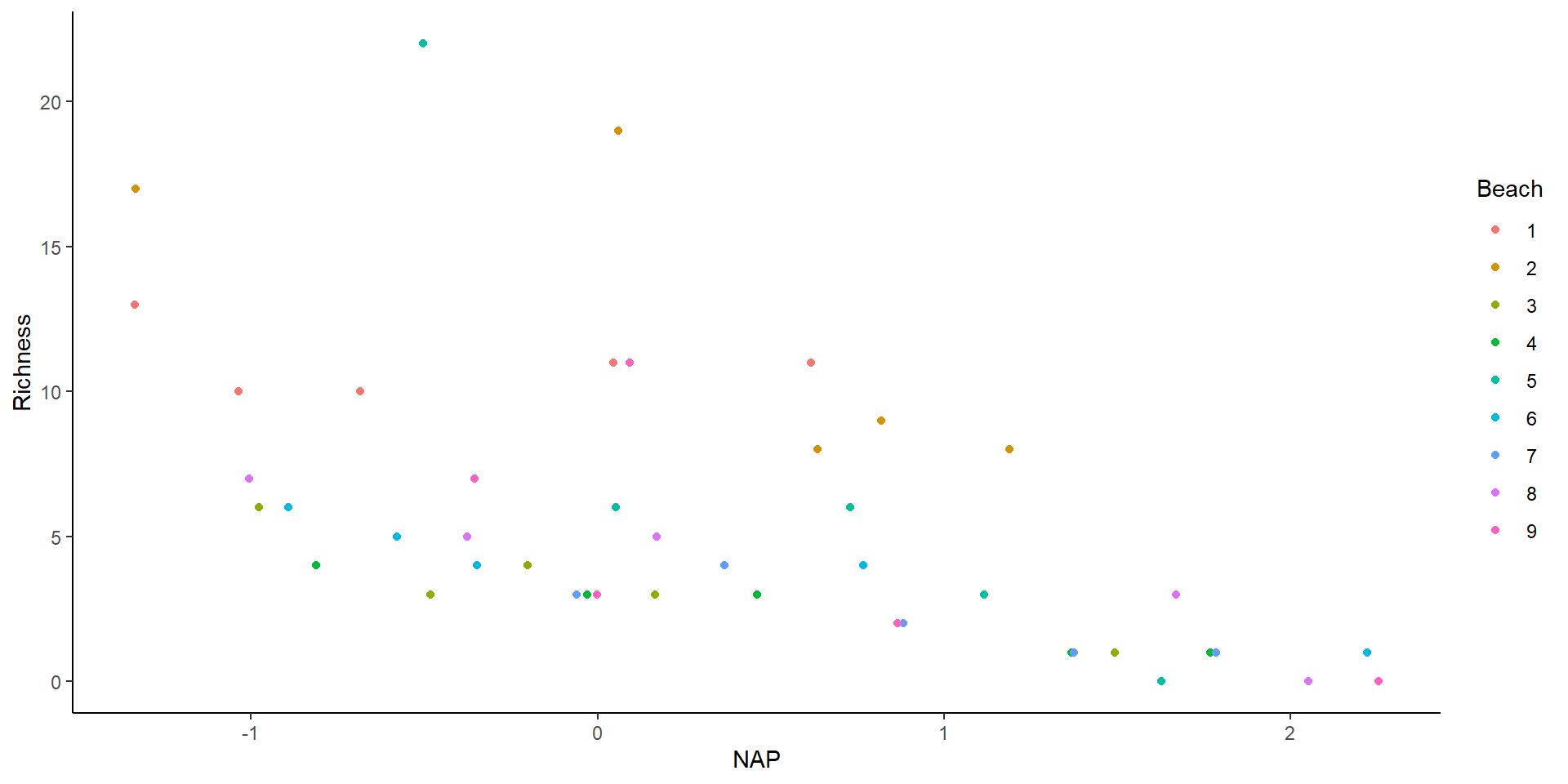
The data
The data
There seems to be an effect of NAP…
how about… a random effect of beach?
step 3: how do we decide random effects?
step 3: random intercept? Or random slope? Or both? Or non
What do we do?
Exposure is categorical… so no random slope 😃
Model selection with random models
WE CANNOT TEST FIXED AND RANDOM EFFECTS AT THE SAME TIME
Talk about Zuur’s weird non-Poisson, and normal analysis
Model selection with random models
Four models. Run all with glmmTMB
Step 1: install the glmmTMB package
Model selection with random models
Fixed effects: NAP*Exposure
Family: Poisson
Model selection based on AICc:

     K   AICc Delta_AICc AICcWt Cum.Wt     LL
Mod1 6 210.94       0.00   0.62   0.62 -98.36
Mod3 7 213.24       2.30   0.20   0.81 -98.10
Mod2 7 213.52       2.59   0.17   0.98 -98.25
Mod4 9 217.81       6.87   0.02   1.00 -97.33
Are the AIC values the same?
Notes on AIC
I recommend using the AICcmodavg package and making a list!
library (AICcmodavg)aictab (list (model1,model2,model3,model4))
Next step: let’s explore the model (factors!)
How do you explore the best model?
Let’s look at the summary
Analysis of Deviance Table (Type II Wald chisquare tests)

Response: Richness
               Chisq Df Pr(>Chisq)
NAP          51.7328  1  6.359e-13 ***
Exposure     55.4525  2  9.092e-13 ***
NAP:Exposure  3.5604  2     0.1686
---
Signif. codes:  0 '***' 0.001 '**' 0.01 '*' 0.05 '.' 0.1 ' ' 1
Next step: let’s explore the model (factors!)
Analysis of Deviance Table (Type II Wald chisquare tests)

Response: Richness
               Chisq Df Pr(>Chisq)
NAP          51.7328  1  6.359e-13 ***
Exposure     55.4525  2  9.092e-13 ***
NAP:Exposure  3.5604  2     0.1686
---
Signif. codes:  0 '***' 0.001 '**' 0.01 '*' 0.05 '.' 0.1 ' ' 1
Talk about Zuur’s approach here
Next step?
<- glm (Richness~ NAP* Exposure, data = rikz, family = poisson)<- glm (Richness~ NAP+ Exposure, data = rikz, family = poisson)<- glm (Richness~ NAP, data = rikz, family = poisson)<- glm (Richness~ Exposure, data = rikz, family = poisson)<- glm (Richness~ 1 , data = rikz, family = poisson)<- AICcmodavg:: aictab (list (model1,model2,model3,model4,model5))
Model selection based on AICc:

     K   AICc Delta_AICc AICcWt Cum.Wt      LL
Mod2 4 209.37       0.00   0.69   0.69 -100.19
Mod1 6 210.94       1.57   0.31   1.00  -98.36
Mod3 2 259.47      50.10   0.00   1.00 -127.59
Mod4 3 265.87      56.50   0.00   1.00 -129.64
Mod5 1 323.84     114.47   0.00   1.00 -160.88
Evidence ratios
Burnham and Anderson
Evidence ratios
Evidence ratio between models 'Mod2' and 'Mod1':
2.19
Last step: Model validation
Of the best model.
Other steps?
Check assumptions (if normal)