Mixed Effects Models

This lecture

Review of linear models

Assumptions of glm’s

Overdispersion

How to interpret GLM’s outputs?

Let’s remember that linear models, and glm’s have a “linear” deterministic component

How to interpret GLM’s outputs?

Let’s remember that linear models, and glm’s have a “linear” deterministic component
In linear models: \(\mu_i = \beta_0 + \beta_1x_{1,i} ...\) (which means, the expected value of y )
In generalized linear models: \(f(\mu_i) = \beta_0 + \beta_1x_{1,i} ...\) (which means, a function of the expected value of y)

The deterministic component is linear

Which is a good thing! Each linear has two components!

A slope
An intercept

The deterministic component is linear

Which is a good thing! Each linear (not polynomial… let’s forget about that for a little while) has two components!

A slope
An intercept

\[ y = mx + b \]

The deterministic component is linear

Which is a good thing! Each linear (not polynomial… let’s forget about that for a little while) has two components!

A slope
An intercept

\[ y = mx + b = b + mx \]

is not any different than:

\[ \begin{align} \mu_i & = \beta_0 + \beta_1x_{1,i} \\ y_i & \sim N(mean = \mu_i, var=\sigma^2) \end{align} \]

Let’s remember what a slope and an intercept is

Slope: For very change in x of 1, y changes 1.5. Intercept: 2
So, if x = 5, then y = 2 + 1.5(5) = 9.5

So, what about linear models?

Each line in a linear model simply has: 1 slope and 1 intercept.

So, what about linear models?

What is the slope? what is the intercept?

So, what about linear models?

\[ \begin{split} y_i & \sim \beta_0 + \beta_1x_i + \epsilon_i \\ \text{where } \epsilon & \sim normal(0,\sigma) \end{split} \] Or, in this specific case:

\[ Reproductive \ effort_i \sim \beta_0 + \beta_1Food \ availability_i + \epsilon_i \\ \]

Intercept and Slope in Linear Models


Call:
lm(formula = ReproductiveEffort ~ Foodavailability, data = foodav)

Residuals:
     Min       1Q   Median       3Q      Max 
-0.37653 -0.25549 -0.04903  0.23662  0.45750 

Coefficients:
                 Estimate Std. Error t value Pr(>|t|)    
(Intercept)       0.89490    0.07262   12.32   <2e-16 ***
Foodavailability  1.19387    0.01590   75.08   <2e-16 ***
---
Signif. codes:  0 '***' 0.001 '**' 0.01 '*' 0.05 '.' 0.1 ' ' 1

Residual standard error: 0.2652 on 61 degrees of freedom
Multiple R-squared:  0.9893,    Adjusted R-squared:  0.9891 
F-statistic:  5636 on 1 and 61 DF,  p-value: < 2.2e-16

Intercept: 0.895
Slope: 1.194

\[ \begin{split} y_i & \sim \beta_0 + \beta_1x_i + \epsilon_i \\ \text{where } \epsilon & \sim normal(0,\sigma) \end{split} \]

Results

Coefficient	Estimate	Std. Error	t-value (test)	p-value
Intercept \(\beta_0\)	0.895
Slope \(\beta_1\)	1.194

\[ \begin{split} y_i & \sim \beta_0 + \beta_1x_i + \epsilon_i \\ \text{where } \epsilon & \sim normal(0,\sigma) \end{split} \]

Results

Coefficient	Estimate	Std. Error	t-value (test)	p-value
Intercept \(\beta_0\)	0.895	0.072	12.32	<0.0001
Slope \(\beta_1\)	1.194	0.0159	75.08	<0.0001

\[ \begin{split} y_i & \sim \beta_0 + \beta_1x_i + \epsilon_i \\ \text{where } \epsilon & \sim normal(0,\sigma) \end{split} \]

Test:
Ho: Coefficient == 0
Ha Coefficient != 0

How about this one:


Call:
lm(formula = FC ~ IC + Dose, data = drugz)

Residuals:
    Min      1Q  Median      3Q     Max 
-2.2610 -0.6360  0.0000  0.6514  2.2876 

Coefficients:
            Estimate Std. Error t value Pr(>|t|)    
(Intercept)  0.51804    0.38892   1.332   0.1849    
IC           0.93384    0.05647  16.537   <2e-16 ***
Dosedose1   -0.44007    0.20011  -2.199   0.0294 *  
Dosedose2   -2.09915    0.20162 -10.412   <2e-16 ***
---
Signif. codes:  0 '***' 0.001 '**' 0.01 '*' 0.05 '.' 0.1 ' ' 1

Residual standard error: 0.9893 on 146 degrees of freedom
Multiple R-squared:  0.7636,    Adjusted R-squared:  0.7588 
F-statistic: 157.2 on 3 and 146 DF,  p-value: < 2.2e-16

Additive model means only one slope is estimated!

Back to the plot

Parallel lines
1 slope, 3 intercepts
Each line: \(y = mx + b\)

Finding values


Call:
lm(formula = FC ~ IC + Dose, data = drugz)

Residuals:
    Min      1Q  Median      3Q     Max 
-2.2610 -0.6360  0.0000  0.6514  2.2876 

Coefficients:
            Estimate Std. Error t value Pr(>|t|)    
(Intercept)  0.51804    0.38892   1.332   0.1849    
IC           0.93384    0.05647  16.537   <2e-16 ***
Dosedose1   -0.44007    0.20011  -2.199   0.0294 *  
Dosedose2   -2.09915    0.20162 -10.412   <2e-16 ***
---
Signif. codes:  0 '***' 0.001 '**' 0.01 '*' 0.05 '.' 0.1 ' ' 1

Residual standard error: 0.9893 on 146 degrees of freedom
Multiple R-squared:  0.7636,    Adjusted R-squared:  0.7588 
F-statistic: 157.2 on 3 and 146 DF,  p-value: < 2.2e-16

\[ \begin{align} \beta_0 & = 0.51 \ \text{intercept for control} \\ \beta_1 & = 0.93 \ \text{slope} \\ \beta_2 & = -0.44 \ \text{Difference in intercept between control and dose 1} \\ \beta_2 & = -2.099 \ \text{Difference in intercept between control and dose 2} \\ \end{align} \]

\[ y_i \sim \beta_0 + \beta_1x_{1,i} + \beta_2x_{2,i} + \beta_3x_{3,i} + \epsilon_i \\ \]

Site	Value of \(x_2\)	Value of \(x_3\)
Control	0	0
Dose 1	1	0
Dose 2	0	1

Finding values


Call:
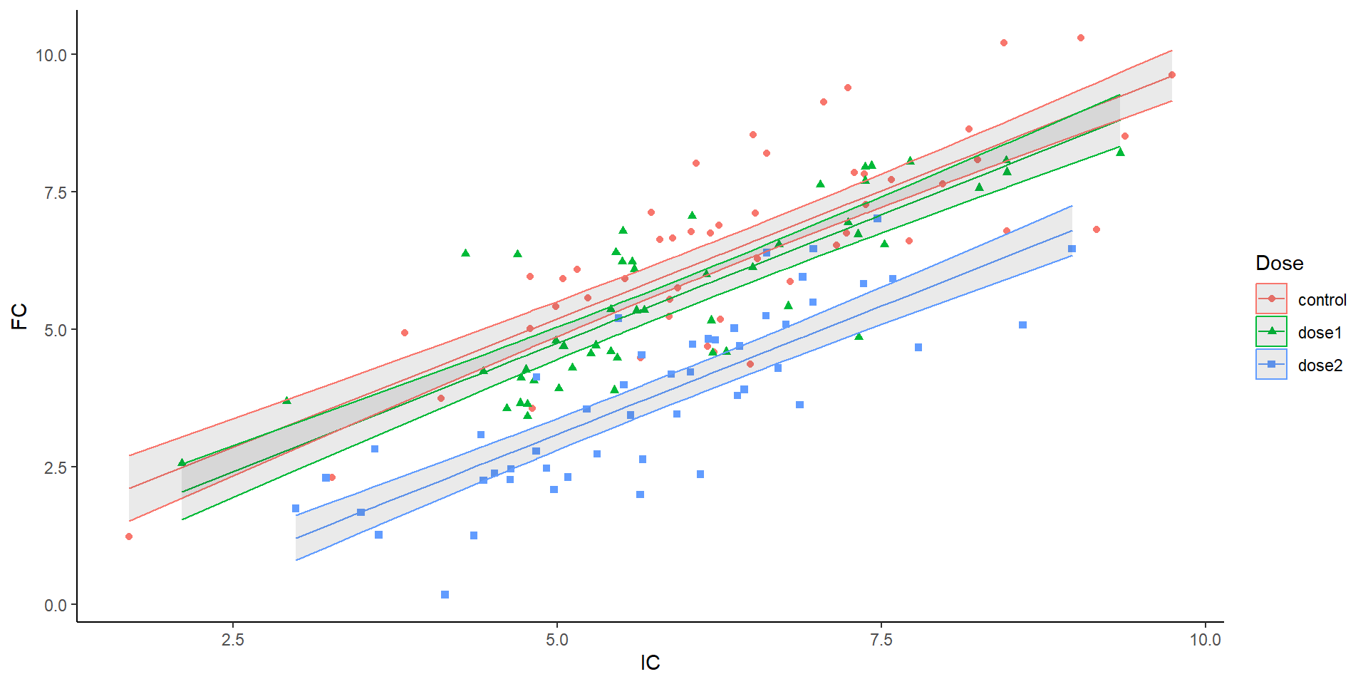
lm(formula = FC ~ IC + Dose, data = drugz)

Residuals:
    Min      1Q  Median      3Q     Max 
-2.2610 -0.6360  0.0000  0.6514  2.2876 

Coefficients:
            Estimate Std. Error t value Pr(>|t|)    
(Intercept)  0.51804    0.38892   1.332   0.1849    
IC           0.93384    0.05647  16.537   <2e-16 ***
Dosedose1   -0.44007    0.20011  -2.199   0.0294 *  
Dosedose2   -2.09915    0.20162 -10.412   <2e-16 ***
---
Signif. codes:  0 '***' 0.001 '**' 0.01 '*' 0.05 '.' 0.1 ' ' 1

Residual standard error: 0.9893 on 146 degrees of freedom
Multiple R-squared:  0.7636,    Adjusted R-squared:  0.7588 
F-statistic: 157.2 on 3 and 146 DF,  p-value: < 2.2e-16

Measurement	Intercept	Slope
Control	0.51	0.93
Dose 1	0.51 - 0.44	0.93
Dose 2	0.51 -2.099	0.93

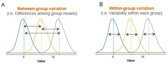
Statistical inference

anova

emmeans

contrast

Analysis of Variance Table

Response: FC
           Df Sum Sq Mean Sq F value    Pr(>F)    
IC          1 342.36  342.36 349.825 < 2.2e-16 ***
Dose        2 119.30   59.65  60.949 < 2.2e-16 ***
Residuals 146 142.89    0.98                      
---
Signif. codes:  0 '***' 0.001 '**' 0.01 '*' 0.05 '.' 0.1 ' ' 1

 contrast        estimate    SE  df t.ratio p.value
 control - dose1     0.44 0.200 146   2.199  0.0747
 control - dose2     2.10 0.202 146  10.412  <.0001
 dose1 - dose2       1.66 0.198 146   8.377  <.0001

P value adjustment: tukey method for comparing a family of 3 estimates

statistical inference

anova compares variance. Is the variance between groups higher than within groups?

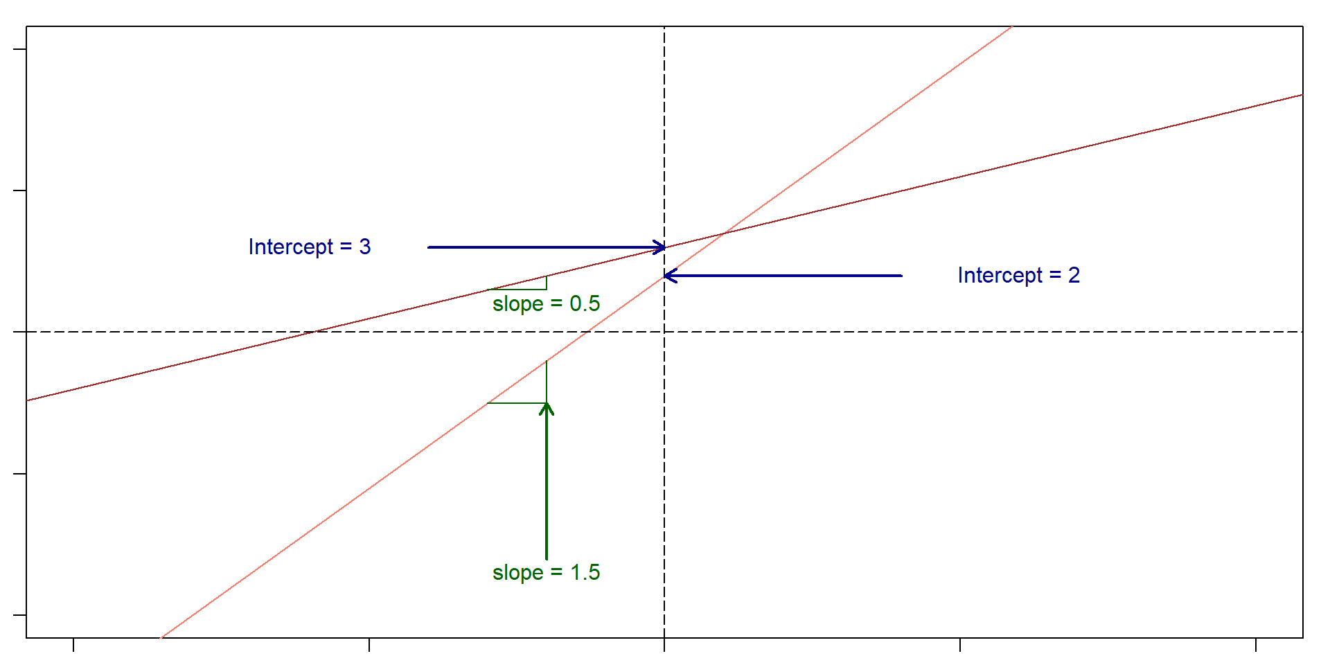
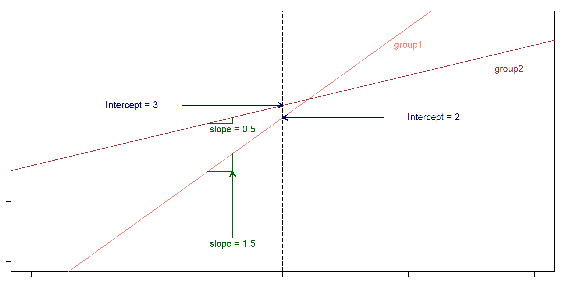
Interactive

Each line has its own slope and its own intercept

Interactive


Call:
lm(formula = FC ~ IC * Dose, data = drugz)

Residuals:
    Min      1Q  Median      3Q     Max 
-2.3167 -0.6262 -0.0031  0.6443  2.1836 

Coefficients:
             Estimate Std. Error t value Pr(>|t|)    
(Intercept)   0.38733    0.59401   0.652   0.5154    
IC            0.95418    0.08981  10.624   <2e-16 ***
Dosedose1     0.07353    0.85237   0.086   0.9314    
Dosedose2    -2.21858    0.86308  -2.571   0.0112 *  
IC:Dosedose1 -0.08529    0.13509  -0.631   0.5288    
IC:Dosedose2  0.02324    0.13917   0.167   0.8676    
---
Signif. codes:  0 '***' 0.001 '**' 0.01 '*' 0.05 '.' 0.1 ' ' 1

Residual standard error: 0.9939 on 144 degrees of freedom
Multiple R-squared:  0.7647,    Adjusted R-squared:  0.7565 
F-statistic: 93.59 on 5 and 144 DF,  p-value: < 2.2e-16

\[ \begin{align} \beta_0 & = 0.38 \ \text{intercept for control} \\ \beta_1 & = 0.954 \ \text{slope for control} \\ \beta_2 & = -0.073 \ \text{Difference in intercept between control and dose 1} \\ \beta_3 & = -2.24 \ \text{Difference in intercept between control and dose 2} \\ \beta_4 & = -0.085 \ \text{Difference in slope between control and dose 1} \\ \beta_5 & = 0.023 \ \text{Difference in slope between control and dose 2} \\ \end{align} \]

Site	Value of \(x_2\)	Value of \(x_3\)	Value of \(x_4\)	Value of \(x_5\)
Control	0	0	0	0
Dose 1	1	0	1	0
Dose 2	0	1	0	1

Doing inference of interactions

Analysis of Variance Table

Response: FC
           Df Sum Sq Mean Sq  F value Pr(>F)    
IC          1 342.36  342.36 346.5514 <2e-16 ***
Dose        2 119.30   59.65  60.3790 <2e-16 ***
IC:Dose     2   0.63    0.31   0.3168  0.729    
Residuals 144 142.26    0.99                    
---
Signif. codes:  0 '***' 0.001 '**' 0.01 '*' 0.05 '.' 0.1 ' ' 1

NOTE: Results may be misleading due to involvement in interactions

 contrast        estimate    SE  df t.ratio p.value
 control - dose1     0.44 0.202 144   2.173  0.0794
 control - dose2     2.08 0.204 144  10.175  <.0001
 dose1 - dose2       1.64 0.201 144   8.136  <.0001

P value adjustment: tukey method for comparing a family of 3 estimates

Interactions

Finding values (predictions)

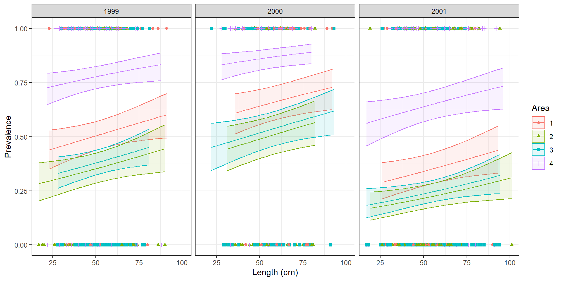
Assignment question 1 📝

Look at the summary. And before continuing make sure you understand it. If you don’t, now is the time to raise your hand.

You need to calculate the expected probability (we’ll call this \(\pi\)) of an individual being infected for each of the following two cases:

An individual of length 50 from Area 1, in 1999
An individual of length 50 from Area 3, in 2001

GLM

Model


Call:
glm(formula = Prevalence ~ Length + Year + Area, family = binomial(link = "logit"), 
    data = cod)

Coefficients:
             Estimate Std. Error z value Pr(>|z|)    
(Intercept) -0.465947   0.269333  -1.730 0.083629 .  
Length       0.009654   0.004468   2.161 0.030705 *  
Year2000     0.566536   0.169715   3.338 0.000843 ***
Year2001    -0.680315   0.140175  -4.853 1.21e-06 ***
Area2       -0.626192   0.186617  -3.355 0.000792 ***
Area3       -0.510470   0.163396  -3.124 0.001783 ** 
Area4        1.233878   0.184652   6.682 2.35e-11 ***
---
Signif. codes:  0 '***' 0.001 '**' 0.01 '*' 0.05 '.' 0.1 ' ' 1

(Dispersion parameter for binomial family taken to be 1)

    Null deviance: 1727.8  on 1247  degrees of freedom
Residual deviance: 1537.6  on 1241  degrees of freedom
  (6 observations deleted due to missingness)
AIC: 1551.6

Number of Fisher Scoring iterations: 4

These are all from a linear model. Need to transform them to get the real value in probabilistic scale

Additive! One slope

How to estimate the values?


Call:
glm(formula = Prevalence ~ Length + Year + Area, family = binomial(link = "logit"), 
    data = cod)

Coefficients:
             Estimate Std. Error z value Pr(>|z|)    
(Intercept) -0.465947   0.269333  -1.730 0.083629 .  
Length       0.009654   0.004468   2.161 0.030705 *  
Year2000     0.566536   0.169715   3.338 0.000843 ***
Year2001    -0.680315   0.140175  -4.853 1.21e-06 ***
Area2       -0.626192   0.186617  -3.355 0.000792 ***
Area3       -0.510470   0.163396  -3.124 0.001783 ** 
Area4        1.233878   0.184652   6.682 2.35e-11 ***
---
Signif. codes:  0 '***' 0.001 '**' 0.01 '*' 0.05 '.' 0.1 ' ' 1

(Dispersion parameter for binomial family taken to be 1)

    Null deviance: 1727.8  on 1247  degrees of freedom
Residual deviance: 1537.6  on 1241  degrees of freedom
  (6 observations deleted due to missingness)
AIC: 1551.6

Number of Fisher Scoring iterations: 4

\[ logistic(\pi_i) = \beta_0 + \beta_1 x_{1,i}+ \beta_2 x_{2,i} + \beta_3 x_{3,i}+ \beta_4 x_{4,i} + \beta_5 x_{5,i} + \beta_6 x_{6,i} \]

Site

	Value of \(x_2\)	Value of \(x_3\)	Value of \(x_4\)	Value of \(x_5\)	Value of \(x_6\)	Value of \(x_7\)
	2000	2001	Area 1	Area 2	Area 3	Area 4
Area-1 1999	0	0	0	0	0	0
Area-1 2000	1	0	0	0	0	0
Area-1 2001	0	1	0	0	0	0
Area-2 1999	0	0	0	1	0	0
Area-2 2000	0	1	0	1	0	0
Area-2 2001	0	0	1	1	0	0
Area 3- 1999	0	0	0	0	1	0
Area 3 -2000	1	0	0	0	1	0
Area 3 - 2001	0	1	0	0	1	0
Area 4 - 1999	0	0	0	0	0	1
Area 4 - 2000	0	1	0	0	0	1
Area 4 2001	0	0	1	0	0	1

Logistic regression assumptions

Binomial distribution
Binary data (1, 0)

Poisson assumptions

We have talked about count-data
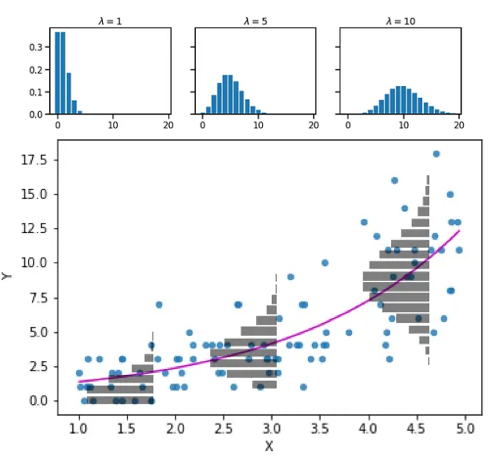
While we usually think Poisson, it has an important assumption: \(Var(y_i) = \lambda\_i\)

How to check for overdispersion?

Package: performance

 performance::check_overdispersion(model)

What to do when there is overdispersion?

I have never encountered non-overdispersed count data!

So, what to do?

Add more covariates
Make a mixed effects model
Zero inflated models!

performance::check_zeroinflation(fit.pr)

What to do when there is overdispersion?

If we suspect zero inflation, we have several options for zero inflated models

Negative binomial regression
Hurdle models
Zero-inflated mixture model (mixed-effects)

GLM’s other assumptions

Data is independently distributed
Error is independent

Question 1

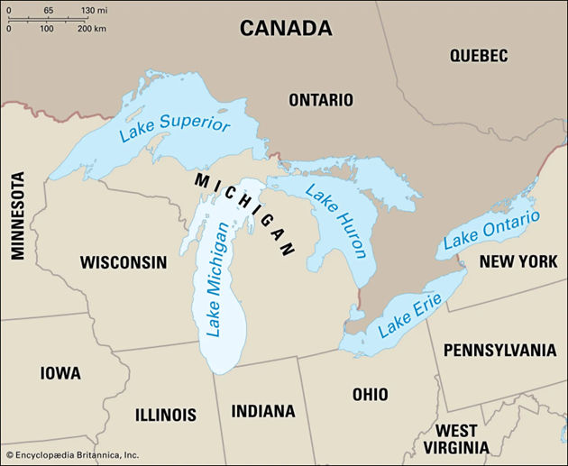
Interested in the concentration of mercury in Lake Michigan

We use code to randomly select 4 sites
At each site we set up a net
Return later and test Hg concentration of each fish

Question 1:

What is the experimental unit?
What is the response variable?
Where is sampling coming from or being introduced?
What do we care about?

Question 2:

We are testing infection prevalence in turkeys 🦃
We trap multiple individuals from a flock, and test them all 🦃
We do this for multiple flocks
What is introducing variance?

Question 3

We are testing the effects of a new drug on mice
You have 100 🐁. And three groups: control, dose 1 and dose 2
You measure their heartbeat pre-trial, 5 weeks post trial, and 10 weeks post trial
Do we care about individual 🐭 or the general effect of the drug?

Question 4

Government is studying how quickly people return to work after receiving unemployment benefits at a national level based on their educational level
Each observation is an individual
Response variables are duartion of benefit, and explanatory variables are education, and industry
You randomly select 25 regional offices to obtain the data
We want to know national levels, but do regional differences matter?

Research Questions

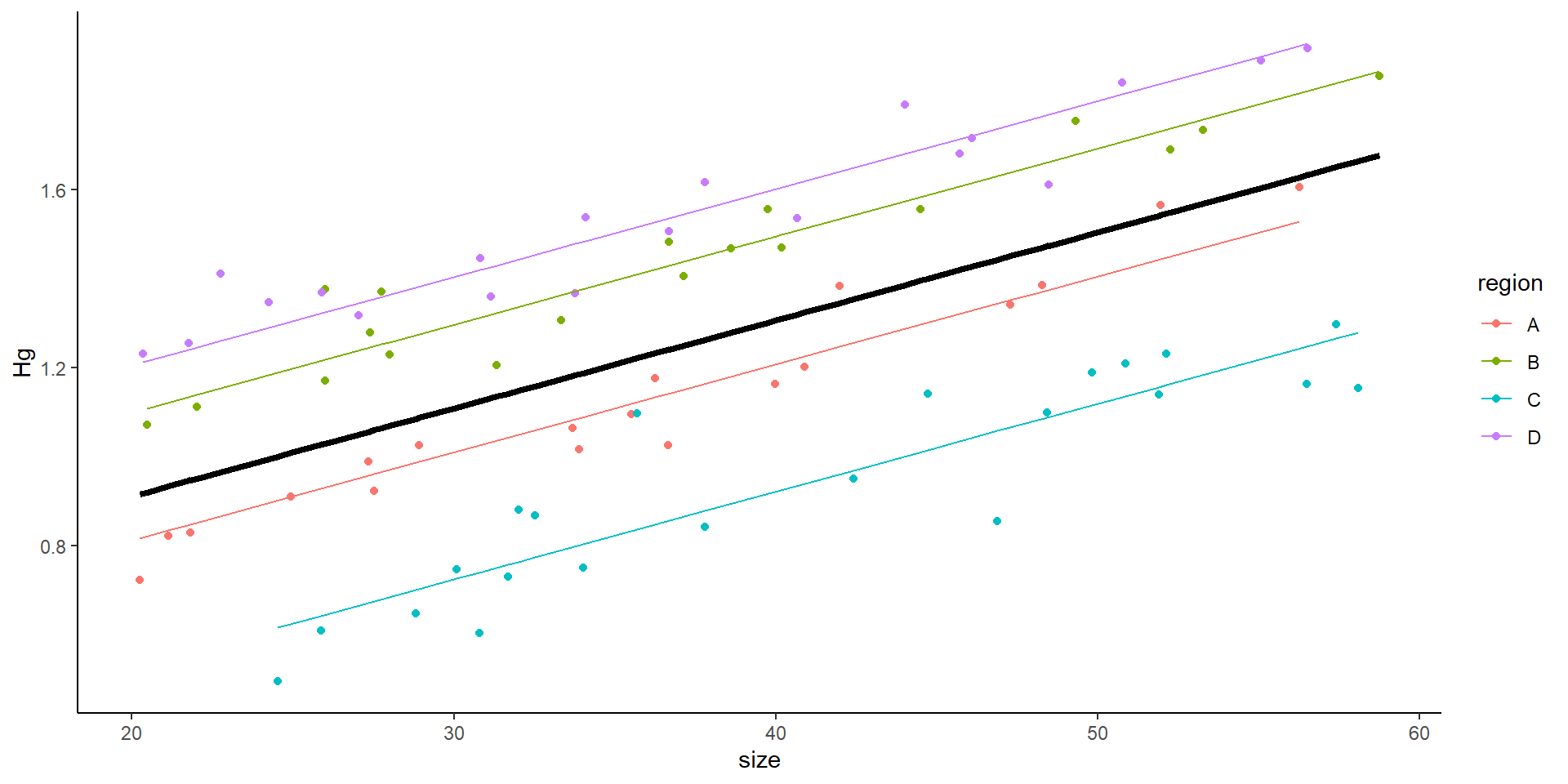
Fish and Hg. Research question: Should we limit consumption of fish over a certain size
Infection prevalence in turkeys: Research question: You are estimating the probability of an individual being infected to be used as a section on a demographic model?
Mice. Research question:Is the drug affecting the mice heart rate?
People Research question: How does educational level affect unemployment time?

Experiments : 🎣 🦃 🐁🧑‍🏭

For one experiment answer:

How would you analyze the data
Are they breaking any assumptions???
What is the individual unit, and what is the experimental unit
What is the response variable
Where is the variance coming from?

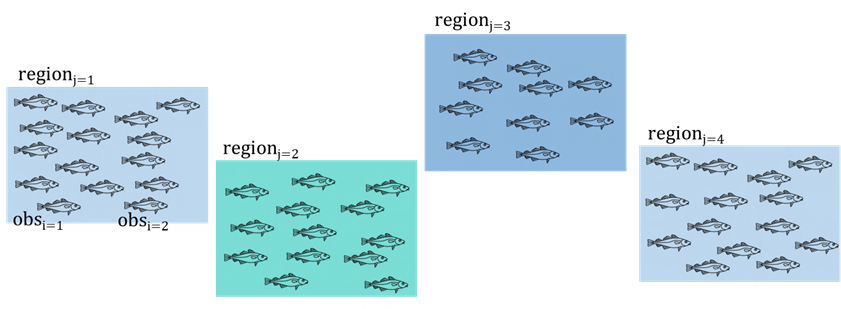
Example 1:

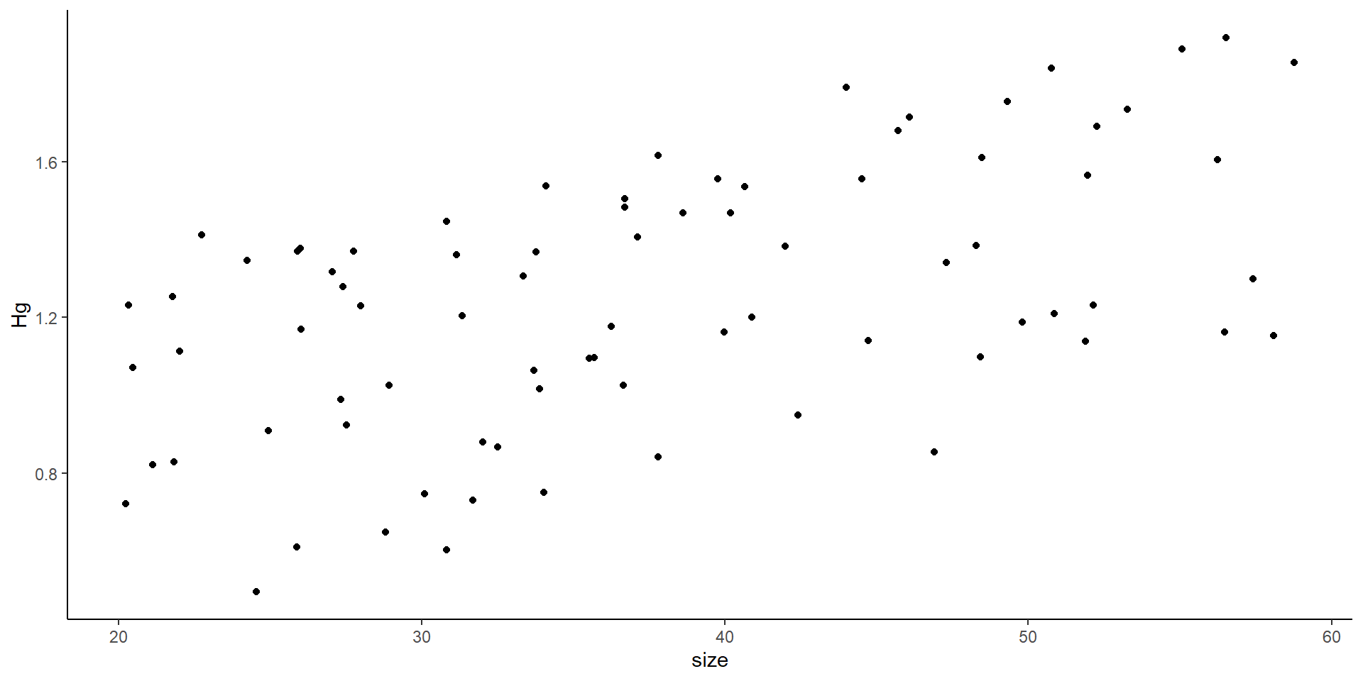
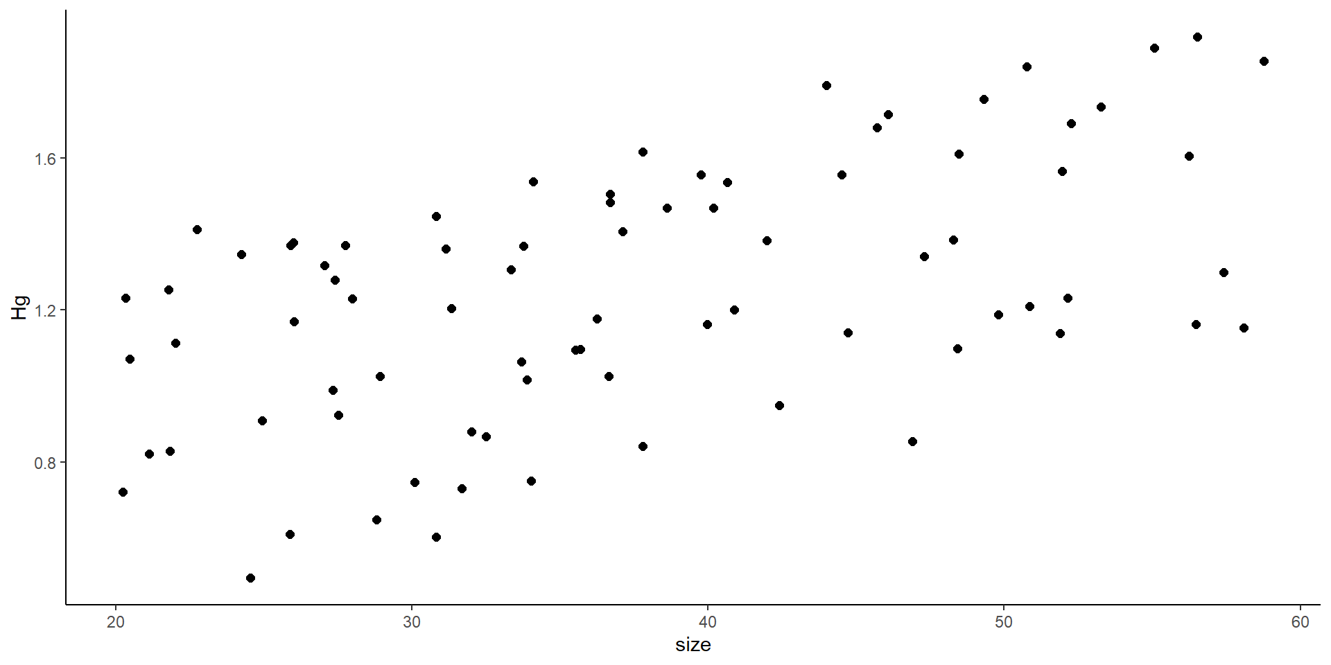
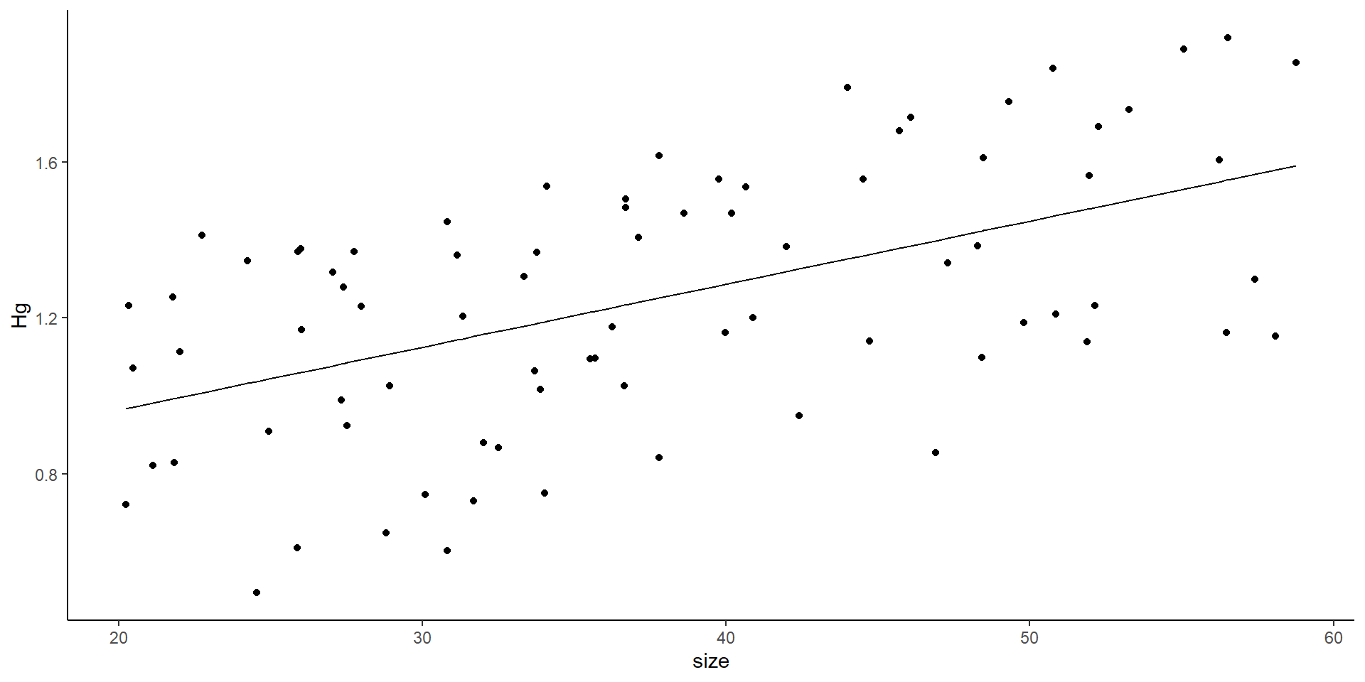
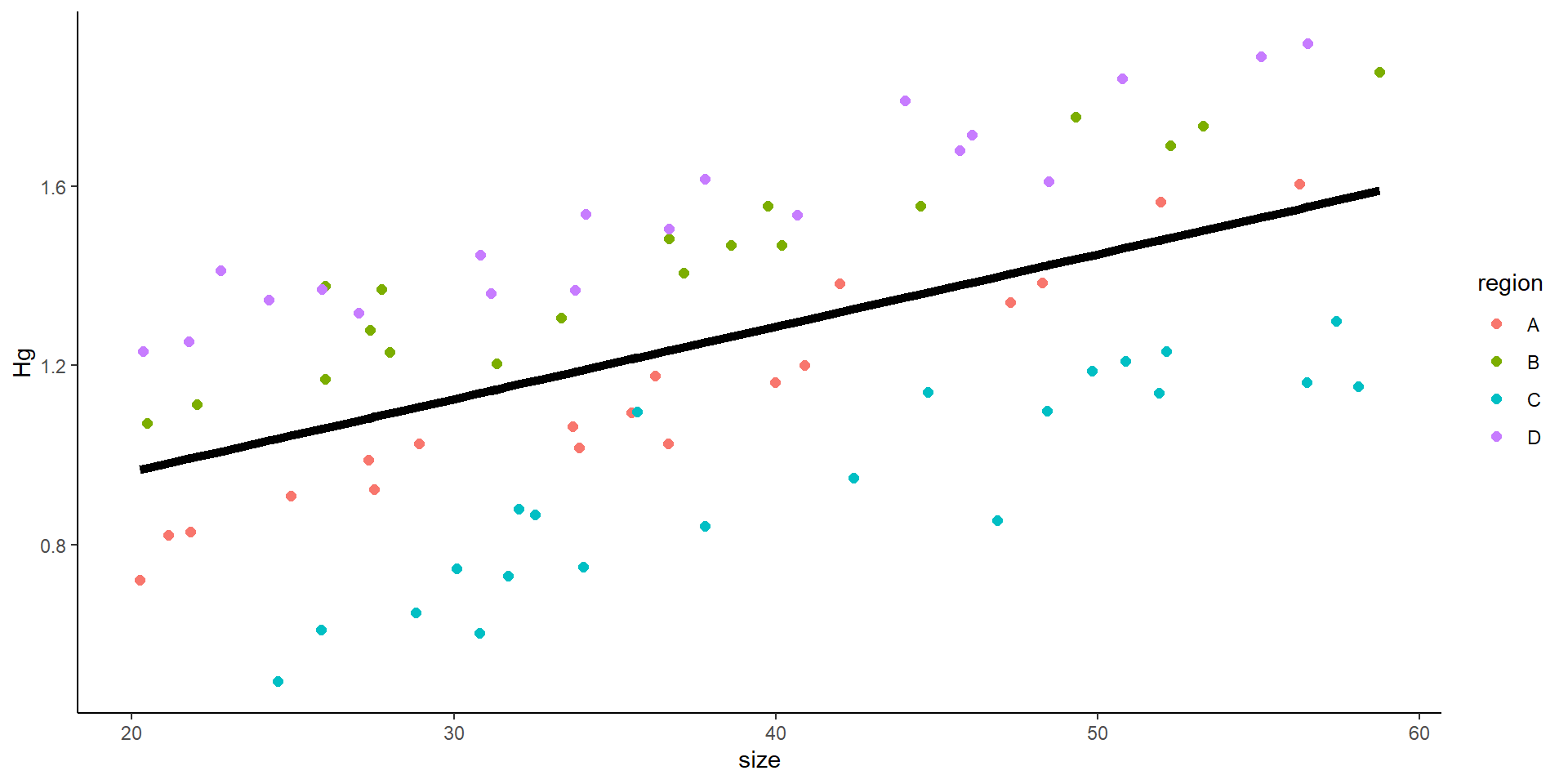
In the first example, we are looking at the relationship between size and Hg concentration, in order to know whether to publish a consumption advisory for fish over a certain size. So, far, we have looked at examples in which our sampling is “random”

      size        Hg ind
1 41.99086 1.3827550   1
2 33.89565 1.0172009   2
3 51.96077 1.5652670   3
4 20.23337 0.7227433   4
5 21.82249 0.8296023   5
6 21.12350 0.8224048   6

Could we simply look at it as
\[ Hg_i \sim \beta_0 + \beta_1 + \epsilon \]

Example 1:

But now the data looks like this:

       size        Hg region ind
1  41.99086 1.3827550      A   1
2  33.89565 1.0172009      A   2
3  51.96077 1.5652670      A   3
25 40.18645 1.4688691      B  25
26 37.12595 1.4055383      B  26
27 20.46721 1.0708612      B  27
56 49.80884 1.1882948      C  56
57 42.40157 0.9499704      C  57
80 56.51251 1.9176455      D  80
NA       NA        NA   <NA>  NA

How do we analyze it?

So far we have looked at linear models (or glms)

\[ \underbrace{E[y_i]}_{\text{expected value}} = \underbrace{\beta_0 + \beta_1x_{1,i} + ... \beta_mx_{m,i}}_{deterministic} \]
\[ y_i \sim \underbrace{N(mean=E[y_i], var=\sigma^2)}_{stochastic} \]
Same as:
\[ y_i = \underbrace{\beta_0 + \beta_1x_{1,i} + ... \beta_mx_{m,i}}_{deterministic} \ + \underbrace{\epsilon}_{stachastic} \]
\[\epsilon \sim nomral(0,\sigma) \]

linear model

\[ \underbrace{E[y_i]}_{\text{expected value}} = \underbrace{\beta_0 + \beta_1x_{1,i} + ... \beta_mx_{m,i}}_{deterministic} \]

\[ y_i \sim \underbrace{N(mean=E[y_i], var=\sigma^2)}_{stochastic} \]

Stochastic portion of a model

When we talk about the stochastic portion of a model:

\[ y_i \sim \underbrace{\beta_0 + \beta_1x_{1,i} + ... \beta_mx_{m,i}}_{deterministic} \ + \underbrace{\epsilon}_{stochastic} \]
What is introducing the variance?
Is the variance (or observation error) independent?
It is unexplained variance!
🎣 🦃 🐁🧑‍🏭
Is the variance unexplained?

Mixed model

Think… how do we introduce that variance?

\[ y_i \sim \underbrace{\beta_0 + \beta_1x_{1,i} + ... \beta_mx_{m,i}}_{deterministic} \ + \underbrace{\epsilon}_{stachastic} \]

Think for a moment on this specific question: 🐟
\[ y_i \sim \underbrace{\beta_0 + \beta_1x_{1,i}}_{deterministic} + \underbrace{\epsilon}_{stachastic} \]
\[ Hg_i \sim \underbrace{\beta_0 + \beta_1size_{i}}_{deterministic} + \underbrace{\epsilon}_{stachastic} \]
\[ \epsilon \sim N(0,\sigma)\]

The variance can affect the slope, the intercept, or both

What is the problem with this? We can actually do a linear model

But remember! there might be some effect of the locations where nets were placed

Plotting the data as a linear model

You might think this is all good… but

So… we do a mixed model! Where we introduce the variance from the site
But… why don’t we simply add site as a covariate?
You will be tasked with answering this on your next assignment!

The variance can affect the slope, the intercept, or both

Random effects introduce variance.
It can introduce varianceto the intercept or to the slope

Mixed model

\[ Hg_i \sim \beta_0 + \beta_1size_{i} + \epsilon \]
i individuals, j sites (4)
\[ Hg_i \sim \underbrace{(\beta_0 +\underbrace{\gamma_j}_{\text{Random intercept}})}_{intercept} + \underbrace{\beta_1size_{i}}_{slope} +\underbrace{\epsilon}_\text{ind var} \]
Variance comes from random “selection” of fish within a net
Variance comes from random “selection” of sites

Mixed model

This is the result of a mixed model:

Mixed effects model output

 Family: gaussian  ( identity )
Formula:          Hg ~ size + (1 | region)
Data: HgDat_df

     AIC      BIC   logLik deviance df.resid 
  -147.6   -138.0     77.8   -155.6       76 

Random effects:

Conditional model:
 Groups   Name        Variance Std.Dev.
 region   (Intercept) 0.070287 0.26512 
 Residual             0.006395 0.07997 
Number of obs: 80, groups:  region, 4

Dispersion estimate for gaussian family (sigma^2): 0.0064 

Conditional model:
             Estimate Std. Error z value Pr(>|z|)    
(Intercept) 0.5160480  0.1364710   3.781 0.000156 ***
size        0.0197595  0.0008332  23.714  < 2e-16 ***
---
Signif. codes:  0 '***' 0.001 '**' 0.01 '*' 0.05 '.' 0.1 ' ' 1

Mixed Effects Models

This lecture

How to interpret GLM’s outputs?

How to interpret GLM’s outputs?

The deterministic component is linear

The deterministic component is linear

The deterministic component is linear

Let’s remember what a slope and an intercept is

Let’s remember what a slope and an intercept is

Let’s remember what a slope and an intercept is

Let’s remember what a slope and an intercept is

So, what about linear models?

So, what about linear models?

So, what about linear models?

Intercept and Slope in Linear Models

Results

Results

How about this one:

How about this one:

Back to the plot

Finding values

Finding values

Statistical inference

statistical inference

Interactive

Interactive

Doing inference of interactions

Interactions

Finding values (predictions)

GLM

Model

How to estimate the values?

Logistic regression assumptions

Poisson assumptions

How to check for overdispersion?

What to do when there is overdispersion?

What to do when there is overdispersion?

GLM’s other assumptions

Question 1

Question 1:

Question 2:

Question 3

Question 4

Research Questions

Experiments : 🎣 🦃 🐁🧑‍🏭

Example 1:

Example 1:

So far we have looked at linear models (or glms)

linear model

Stochastic portion of a model

Mixed model

The variance can affect the slope, the intercept, or both

Plotting the data as a linear model

The variance can affect the slope, the intercept, or both

Mixed model

Mixed model

Mixed effects model output

Output