Bayesian statistics: part three

SNR 610

Bayesian

  • Gives us a posterior, based on a prior an a Likelihood –> models a probability. It is obtained by the product of:

  • Likelihood, probability of a parameter being something, given our data

  • Prior: the information we had about a system

Challenge. Bats per net

  • You are surveying bats near a beach. You set up one mist net and caught 8 bats

  • From previous surveys, you know that the mean catch per net is around 10 bats, with a standard deviation of around 3 bats

  • Estimate Likelihood, prior, combine them (joint) and estimate the posterior (normalized so that it sums to 1)

  • Plot all three on the same graph: likelihood, prior, and posterior –> Scale the prior and likelihood if necessary so they fit on the same plot

  • Find the most probable value of \(\lambda\)

Step1: Likelihood

What would the first step be?

Lambda=seq(0,22, by=0.1)
Likelihood=dpois(8,Lambda)
plot(Lambda,Likelihood,type="l", col="blue", lwd=2,ylab="Likelihood", xlab="Lambda")

Step 2: Prior

mu <- 10
sigma <- 3

beta <- mu / sigma^2
alpha <- mu * beta

prior <- dgamma(Lambda, shape = alpha, rate = beta)


plot(Lambda,prior,type="l", col="salmon", lwd=2,ylab="Likelihood", xlab="Lambda")
lines(Lambda,Likelihood,, col="blue", lwd=2)

Step 3: Joint

jointL<-prior*Likelihood

Step 4: Posterior and plot

Posterior<- jointL/sum(jointL)
plot(Lambda,Posterior,type="l", lwd=4, lty=2,ylab="joint Likelihood", xlab="Lambda")

Plot them together

plot(Lambda,Posterior,type="l", lwd=4, lty=2,ylab="joint Likelihood", xlab="Lambda")
lines(Lambda,Likelihood, col="blue", lwd=2)
lines(Lambda,prior, col="salmon", lwd=2)

Plot them again

Need scaling

Based on posterior

L_scaled <- Likelihood * max(Posterior) / max(Likelihood)
prior_scaled <- prior * max(Posterior) / max(prior)


plot(Lambda,Posterior,type="l", lwd=4, lty=2,ylab="joint Likelihood", xlab="Lambda")
lines(Lambda,L_scaled, col="blue", lwd=2)
lines(Lambda,prior_scaled, col="salmon", lwd=2)

How do humans think

flowchart LR
  A[Experience] --> B[Observation]
  B --> C[Updated Belief]
  C --> A

Be it human relations, weather, or sports!

  • We do not think about about things in “point estimates” but more distribution like

Comparing methods (Bayesian vs Frequentist)

Assume you have data for 37 night nets, rather than just one. Same prior as before (mean =10 and sd =3)

How would we estimate the posterior?

print(bats)
 [1]  6 12 12 12 14  9  9  9  8  9  7 13 16  5  5  7 14 12  9 13  9  4 11 11  9
[26]  8  4 10  8  3  8 13  5 12  6  7  6

Bayesian

Lambda=seq(0,22, by=0.1)

Likelihood=sapply(Lambda, function(l) prod(dpois(bats, l)))

mu <- 10
sigma <- 3

beta <- mu / sigma^2
alpha <- mu * beta

prior <- dgamma(Lambda, shape = alpha, rate = beta)

jointL<-prior*Likelihood

Posterior<- jointL/sum(jointL)
plot(Lambda,Posterior,type="l", lwd=4, lty=2,ylab="joint Likelihood", xlab="Lambda")

Frequentist

mean(bats)
[1] 9.054054
  • Which one is harder?

Different outputs

Frequentist

One estimate (most likely value; expected value)

Uncertainty is given by Confidence Intervals

Bayesian

A posterior distribution

Represents our updated belief about \(\lambda\)

Uncertainty is both shape and spread!

How about two parameters?

  • Imagine now you have continuous data

  • You have a mean

  • You have variance

  • Bayesian needs a 2-d likelihood surface

What is a 2-d surface

Imagine you want to test the likelihood of \(\mu\) from 70 to 80

You want to tests the likelihood of \(\sigma\) from 3 to 7

Each time you run a likelihood estimate you run a joint likelihood of both mean and sd and you want to test all potential combinations!

For a normal model with data

\[y_i \sim \text{Normal}(\mu, \sigma) \]

We need to explore both parameters:

\[P(\mu, \sigma \mid y) \propto P(y \mid \mu, \sigma) \times P(\mu, \sigma) \]

Frequentist:
- Closed-form solutions
\[\hat{\mu} = \bar{y} \\ \hat{\sigma} = \text{sd}(\bar{y})\]

Bayesian:
- Must compute (or sample) over the entire 2D surface!

set.seed(123)
y <- rnorm(20, mean = 75, sd = sqrt(22))

# Define grid for mu and sigma
mu_vals <- seq(70, 80, by=0.01 )
sigma_vals <- seq(3, 7, by=0.01)

# Compute log-likelihood surface
ll <- outer(mu_vals, sigma_vals, Vectorize(function(mu, sigma) {
  sum(dnorm(y, mean = mu, sd = sigma, log = TRUE))
}))

# Convert to likelihood
lik <- exp(ll - max(ll))  # rescale for plotting

Plot

# Contour plot of the 2D likelihood surface

contour(mu_vals, sigma_vals, lik,
xlab = expression(mu), ylab = expression(sigma),
main = "2D Likelihood Surface")
points(mean(y), sd(y), col = "red", pch = 19)
text(mean(y), sd(y), "MLE", pos = 4, col = "red")

Takeaway

  • In Bayesian, if we are doing one estimate (\(\lambda\)) we can do a curve

  • If we are doing two estimates, we need a contour plot, or a surface plot

  • For two estimates we have essentially a matrix

  • More than two estimates?

Example

Example from assignment 5

codmodel1<-glm(Prevalence~Length+Year+Area,data=cod,family = binomial(link="logit"))
summary(codmodel1)

Call:
glm(formula = Prevalence ~ Length + Year + Area, family = binomial(link = "logit"), 
    data = cod)

Coefficients:
             Estimate Std. Error z value Pr(>|z|)    
(Intercept) -0.465947   0.269333  -1.730 0.083629 .  
Length       0.009654   0.004468   2.161 0.030705 *  
Year2000     0.566536   0.169715   3.338 0.000843 ***
Year2001    -0.680315   0.140175  -4.853 1.21e-06 ***
Area2       -0.626192   0.186617  -3.355 0.000792 ***
Area3       -0.510470   0.163396  -3.124 0.001783 ** 
Area4        1.233878   0.184652   6.682 2.35e-11 ***
---
Signif. codes:  0 '***' 0.001 '**' 0.01 '*' 0.05 '.' 0.1 ' ' 1

(Dispersion parameter for binomial family taken to be 1)

    Null deviance: 1727.8  on 1247  degrees of freedom
Residual deviance: 1537.6  on 1241  degrees of freedom
  (6 observations deleted due to missingness)
AIC: 1551.6

Number of Fisher Scoring iterations: 4
  • 7 different estimates!

  • Joint Likelihood for each one!

  • Really hard to choose a starting value!

  • If we get 8 bats, easy to choose a beta. In a model it is hard to choose a beta!

Many parameters

  • Imagine a simple linear model

  • \[ y_i \sim \beta_0 + \beta_1x_{1i} + \beta_2x_{2i} + \beta_3x_{3i} + \epsilon_i \]

  • Posterior: \(P (\beta_0, \beta_1, \beta_2, \sigma | data)\)

  • We cannot make a grid! We cannot visualize!

How do models solve this?

In frequentist: Equations that minimize residuals. It uses calculus and algebra

  • You get the same solution each time. If all of you run the same model with the same data in R, you will all get the same betas as me!

  • Bayesian Integrates a posterior –> No closed solution!

  • Different solution each time!

  • Why? Bayesian cannot solve this using an equation. So, it samples from it using Markov Chain Monte Carlo (MCMC!) and obtains a probability from it

MCMC?

  • Ever heard of this?

  • Let’s try this! With a game!

In-Pairs Exercise: Acting Out an MCMC Random Walk

Goal

Experience how MCMC explores a likelihood surface step-by-step. NO COMPUTER NEEDED!

DO NOT RUN ANYTHING YET!

Choose one student to do the random walk, one to be the computer or tester

Exercise

Goal

Experience how MCMC explores a likelihood surface step-by-step. NO COMPUTER NEEDED!

Setup

  1. Student A: open and run the following code (DO NOT SHOW TO STUDENT B!):
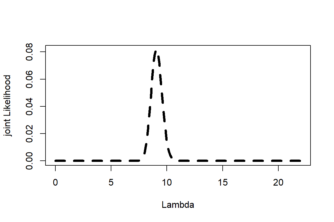
x <- seq(-50, 150, by = 1)

# Create a landscape with 3 peaks of different widths and heights
likelihood <- 
  0.7 * dnorm(x, mean = 20, sd = 10) +
  1.0 * dnorm(x, mean = 80, sd = 15) +
  0.4 * dnorm(x, mean = 120, sd = 5)

# Normalize so it looks like a probability surface
likelihood <- likelihood / max(likelihood)

plot(x, likelihood, type = "l", lwd = 3, col = "darkgreen",
     xlab = "Parameter value (x)",
     ylab = "Relative likelihood",
     main = "Example Likelihood Landscape")
  1. Student B: secretly pick a starting point (between 0 and 100). Call this x

The Walk

  1. Student B: Write down the starting point (x) and mention it to student A. Student A tell student B an approximate value of the Likelihood. Write it down.

  2. Student B: flips a “coin” in R:

rbinom(1, 1, 0.5)
[1] 0

If 1 –> propose x + 3

If 0 –> propose x – 3

  1. Student A: checks the new height (likelihood) and compares it to the current. If new height > current, move 3 steps in that direction (Student B: write down the new x, student A write Likelihood) If not, move only 1 step. Write down the new x and Likelihood as well.

Repeat ~20 times

Plot in paper (x value vs Likelihood)

MCMC

Start with a random guess.

Propose a new set of parameters.

Accept or reject based on how likely they are given the data.

Repeat thousands of times. The chain “learns” the posterior shape.

Youtube video

Gibbs sampler

Most of our software uses a Gibbs sampler.

  • It tests one parameter at a time.

  • Fixes some parameters and moves one around

  • After a while, it switches to a different parameter, and so on

Next classes (suggestion)

  • Wednesday: Plots

  • Friday: A Bayesian example (only for those interested).

  • Next Week: Multivariate (lecture). Friday lab, no need to turn in, but an exercise I want you to do

  • Monday 24: Session to work on final project (no class)

  • Monday 1st. Session to work on final project (no class). Free coffee + snacks (RSVP)!