Bayesian statistics: part two
Bayesian
A different statistical framework
We have used frequentist so far
Parameters
Fixed unknown
Random variable
Data
Random
Fixed
Inference
Based on a sampling distribution
Based on posterior
Output
P-value, Confidence intervals, betas
Credible intervals and posterior distribution
Computational needs
low
high
Bayesian take away
Different way of looking at things… we will explore how
Bayes Theorem
\[
\Huge P(\theta |data) = \frac{P(data|\theta) \times P(\theta)}{P(data)}
\]
\(P(\theta|data)\) : Posterior, probability of theta, given the data\(P(data|\theta)\) : Likelihood! \(\mathcal{L}(\theta|data) = P(data|\theta)\) \(P(\theta)\) : Prior (who knows what this is!)\(P(data)\) : Marginal (who knows!)
Challenges
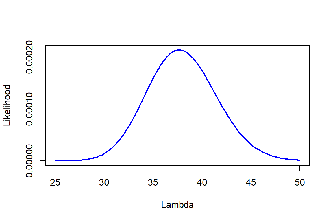
You go out to a Forest that has been separated in multiple plots. You are wondering what the count of total trees per plot is (\(\lambda\) ). You only can count the number of trees in one plot chosen at random. You count 37 trees, Estimate the Likelihood of different values of \(\lambda\) as well as the maximum likelihood.
= seq (25 ,50 , by= 0.25 )= dpois (37 ,Lambda)plot (Lambda,Likelihood,type= "l" , col= "blue" , lwd= 2 ,ylab= "Likelihood" , xlab= "Lambda" )
Answers Q2
= seq (25 ,50 , by= 0.25 )= dpois (37 ,Lambda)* dpois (41 ,Lambda)* dpois (35 ,Lambda)plot (Lambda,Likelihood,type= "l" , col= "blue" , lwd= 2 ,ylab= "Likelihood" , xlab= "Lambda" )
We usually have more than one n
The more data, the better!
= dpois (37 ,Lambda)plot (Lambda,Likelihood,type= "l" , col= "blue" , lwd= 2 ,ylab= "Likelihood" , xlab= "Lambda" )= dpois (37 ,Lambda)* dpois (41 ,Lambda)* dpois (35 ,Lambda)plot (Lambda,Likelihood,type= "l" , col= "blue" , lwd= 2 ,ylab= "Likelihood" , xlab= "Lambda" )
In this case:
\[
\mathcal{L} = P(X_1 = 37 | \lambda) \times P(X_1 = 41 | \lambda) \times P(X_1 = 35 | \lambda)
\]
In general:
\[
\mathcal{L}(x_1, x_2, ...,x_n) = \prod_{i=1}^n P(X_i = x_i | \lambda)
\]
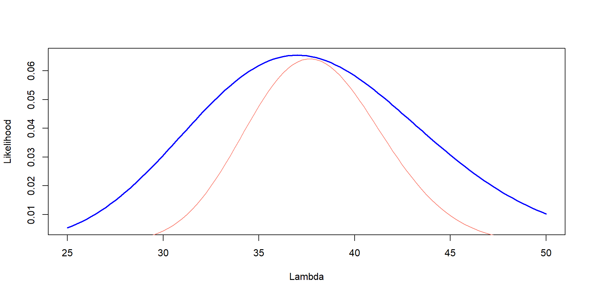
Hard to compare
= dpois (37 ,Lambda)plot (Lambda,Likelihood,type= "l" , col= "blue" , lwd= 2 ,ylab= "Likelihood" , xlab= "Lambda" )= dpois (37 ,Lambda)* dpois (41 ,Lambda)* dpois (35 ,Lambda)lines (Lambda,Likelihood, type= "l" , col= "salmon" )
Hard to compare
= dpois (37 ,Lambda)plot (Lambda,Likelihood,type= "l" , col= "blue" , lwd= 2 ,ylab= "Likelihood" , xlab= "Lambda" )= dpois (37 ,Lambda)* dpois (41 ,Lambda)* dpois (35 ,Lambda)lines (Lambda,Likelihood* 300 , type= "l" , col= "salmon" )
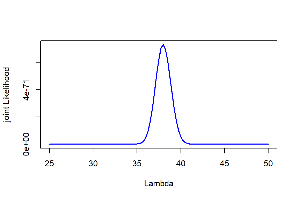
Multiple data
forest object with counts of 50 plots
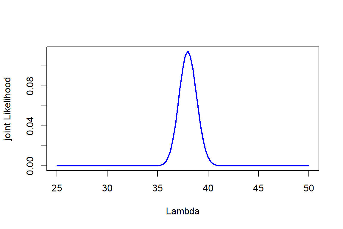
= seq (25 ,50 , by= 0.25 )= sapply (Lambda, function (l) prod (dpois (forest, l)))plot (Lambda,Likelihood,type= "l" , col= "blue" , lwd= 2 ,ylab= "joint Likelihood" , xlab= "Lambda" )
Dealing with tiny numbers
= seq (25 ,50 , by= 0.25 )= sapply (Lambda, function (l) prod (dpois (forest, l)))<- Likelihood/ sum (Likelihood)plot (Lambda,scaled_Likelihood,type= "l" , col= "blue" , lwd= 2 ,ylab= "joint Likelihood" , xlab= "Lambda" )
Bayes Theorem
\[ \Huge P(\theta |data) = \frac{P(data|\theta) \times P(\theta)}{P(data)} \]
\(P(\theta|data)\) : Posterior, probability of theta, given the data\(P(data|\theta)\) : Likelihood! \(\mathcal{L}(\theta|data) = P(data|\theta)\) \(P(\theta)\) : Prior (who knows what this is!)\(P(data)\) : Marginal (who knows!)
Prior
Before talking about priors, I want to tell you all a story
I saw a rabbit
I saw a fox
I saw a cougar
I saw a platypus
Data was the same for all 3
So… Likelihood would be the same.
\[
\mathcal{L}(statement = true\ \ | \ \ \text{my thrustworthy professor told me})
\]
In each of the four cases, I told you I saw it (think of this as data)
So, why did you believe me some times and not other times?
Priors!
Priors
The prior distribution provides un with a way of incorporating information about \(\theta\) (population parameter) in our analysis
In our lives, any new information is weighed with any prior… so you are all Bayesian
Cleveland Browns and Bayesian Thinking
You check the score: the Browns are up 21 to 7 at halftime against the Ravens. In frequentist probability, you would think:
“Probability of winning when going 21-7 is about 80%”
\[ \text{Posterior belief} \propto \text{Prior (they find ways to lose)} \times \text{New data (they’re winning now)} \]
Essentially, you know that they tend to find ways to lose
You may be expecting heartbreak, despite the data (21-7)
Weather
Your weather app says that there is 5% of rain
You get out, and t is overcast, cloudy, and windy… you may get your umbrella
This is based on priors! You know that when the sky looks like that, it usually rains
Where do priors come from?
How to incorporate priors?
\[ \Huge P(\theta |data) = \frac{P(data|\theta) \times P(\theta)}{P(data)} \]
Example
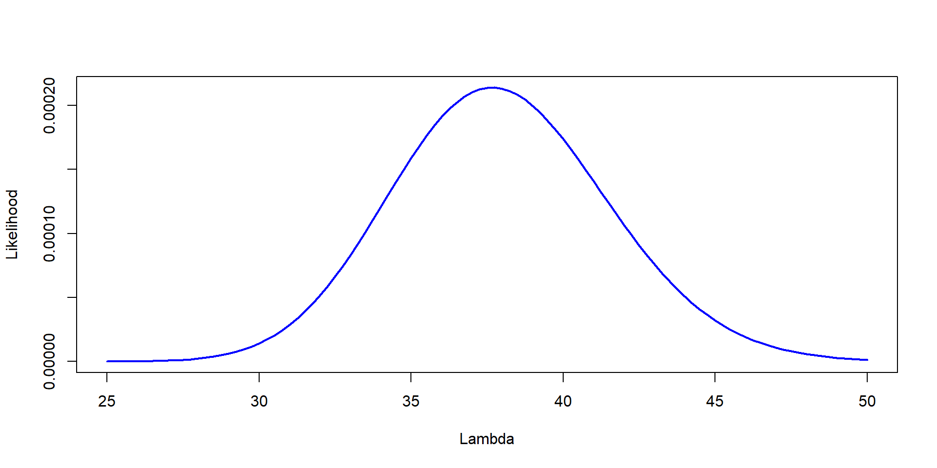
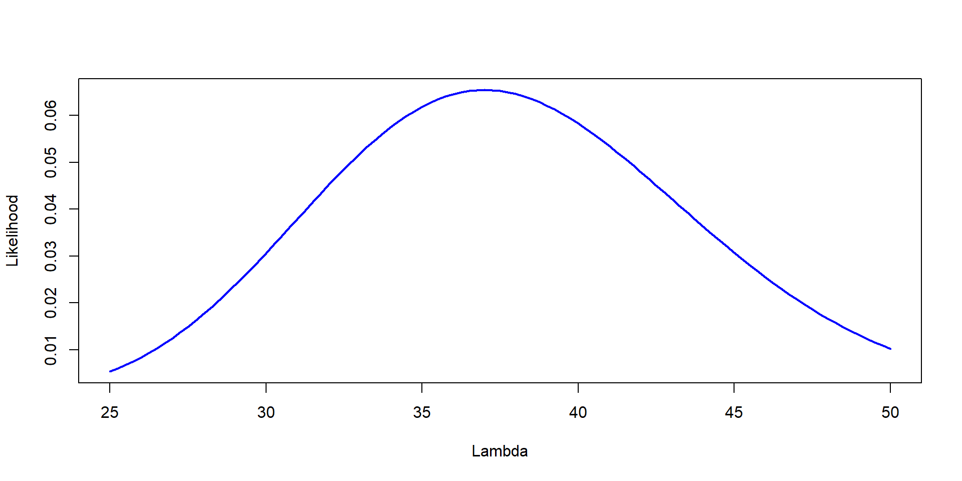
You go to the same Forest, but were able to count three plots. They had 37, 41 and 35 trees. Estimate the Likelihood of different values of \(\lambda\)
= seq (25 ,50 , by= 0.25 )= dpois (37 ,Lambda)* dpois (41 ,Lambda)* dpois (35 ,Lambda)plot (Lambda,Likelihood,type= "l" , col= "blue" , lwd= 2 ,ylab= "Likelihood" , xlab= "Lambda" )
This is the Likelihood
\[ P(\theta | data) = \frac{P(data|\theta) \times P(\theta)}{P(data)} \]
Joint Likelihood: We need to multiply it by the priors
A prior study (one year ago), you counted trees per plots. And found a mean of 39.9 and a sd of 6.75
In this example
Likelihood:
= seq (25 ,50 , by= 0.25 )= dpois (37 ,Lambda)* dpois (41 ,Lambda)* dpois (35 ,Lambda)= Likelihood/ sum (Likelihood)
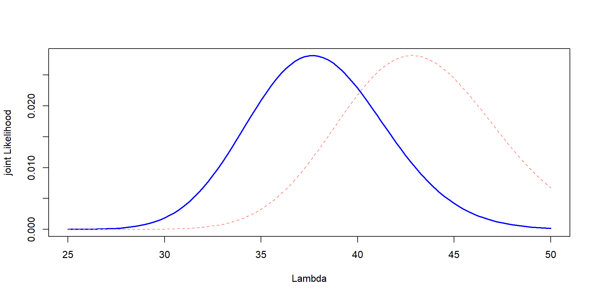
A prior study (one year ago), you counted trees per plots. And found a mean of 43.2 and a sd of 4.05
# Example prior as Gamma <- 43.2 <- 4.05 <- mu / sigma^ 2 <- mu * beta<- dgamma (Lambda, shape = alpha, rate = beta)
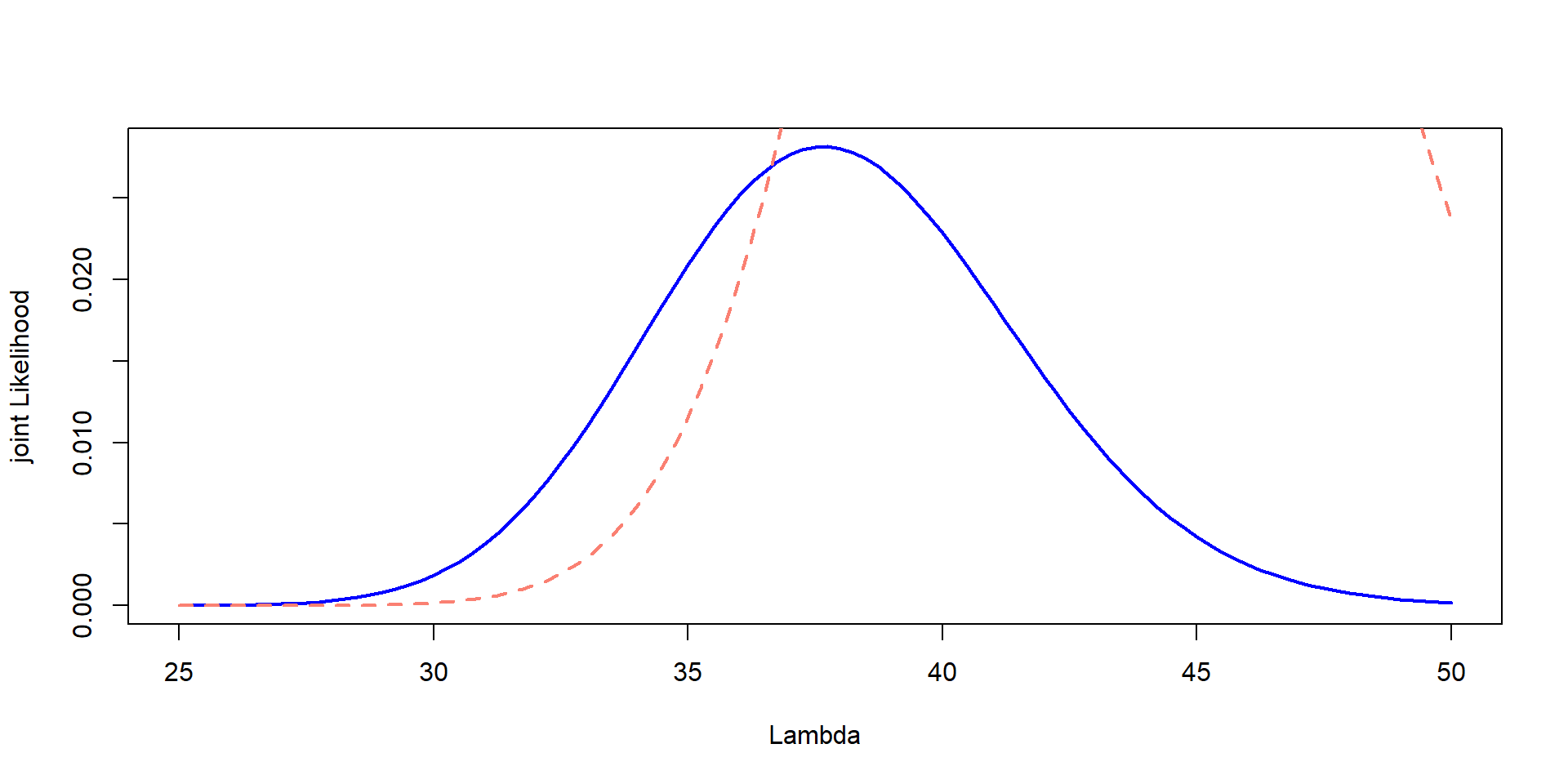
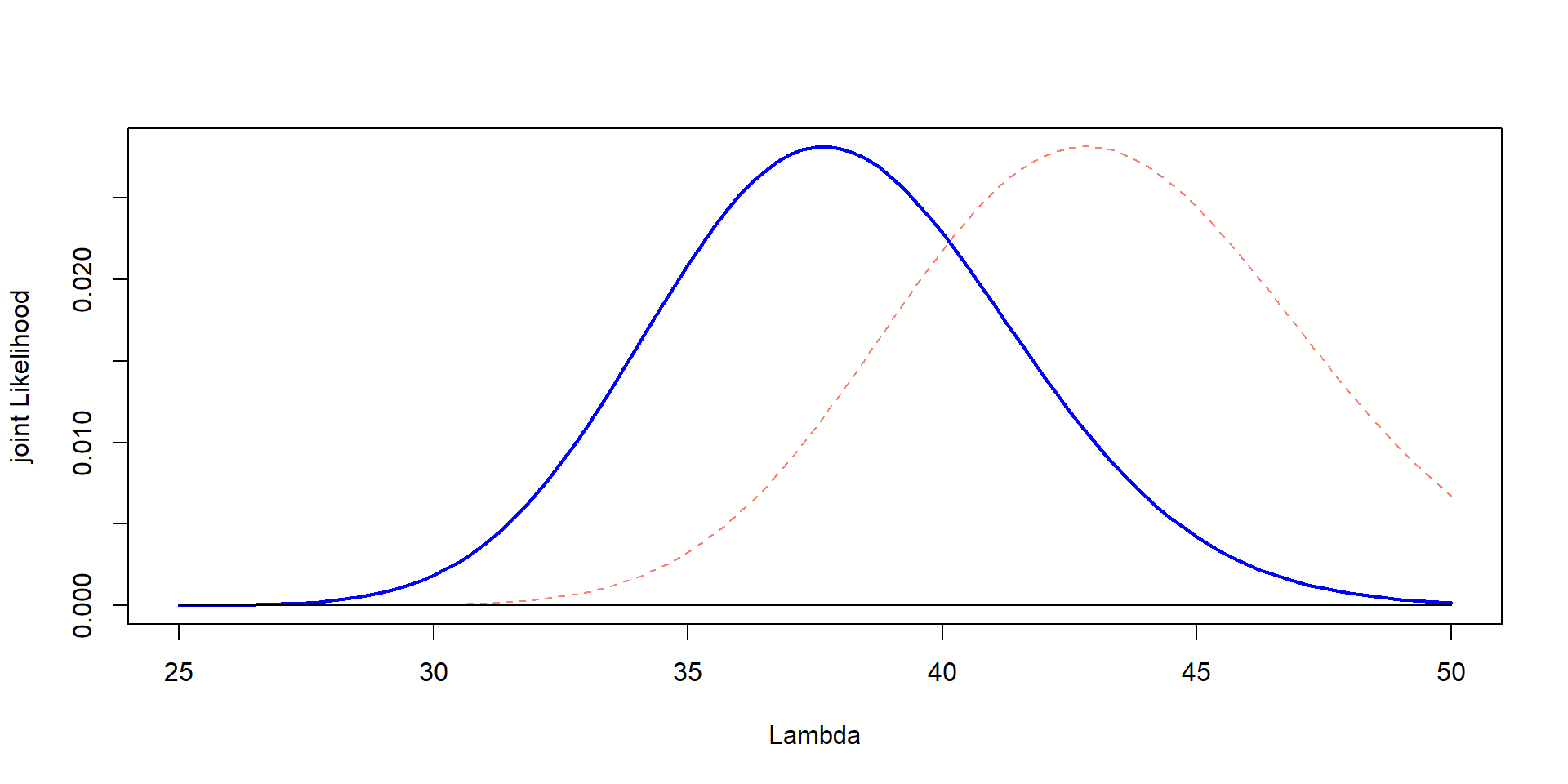
Together
plot (Lambda,Likelihood_scaled,type= "l" , col= "blue" , lwd= 2 ,ylab= "joint Likelihood" , xlab= "Lambda" )lines (Lambda, prior, col= "salmon" , lty= 2 ,lwd= 2 )
<- prior * max (Likelihood_scaled) / max (prior)plot (Lambda,Likelihood_scaled,type= "l" , col= "blue" , lwd= 2 ,ylab= "joint Likelihood" , xlab= "Lambda" )lines (Lambda, prior_scaled, col= "salmon" , lty= 2 )
Joint Likelihood
\[
P(data|\theta) \times P(\theta)
\]
Multiply them! The original numbers!
Scaling is good… but just for plotting, we need to use the actual estimates!
Multiply them
<- prior * Likelihood
That’s it! We have our joint Likelihood!
We cannot plot it
It is in different scales!
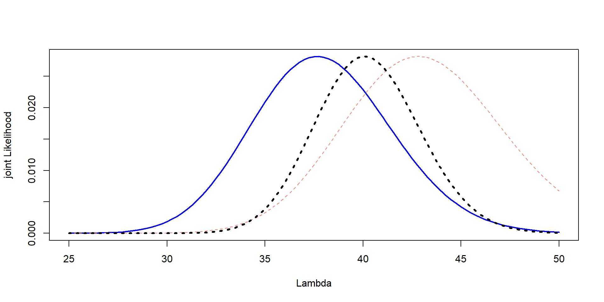
plot (Lambda,Likelihood_scaled,type= "l" , col= "blue" , lwd= 2 ,ylab= "joint Likelihood" , xlab= "Lambda" )lines (Lambda, prior_scaled, col= "salmon" , lty= 2 )lines (Lambda,jointL)
Scale it (for plots)
<- jointL * max (Likelihood_scaled) / max (jointL)<- prior * max (Likelihood_scaled) / max (prior)plot (Lambda,Likelihood_scaled,type= "l" , col= "blue" , lwd= 2 ,ylab= "joint Likelihood" , xlab= "Lambda" )lines (Lambda, prior_scaled, col= "salmon" , lty= 2 )lines (Lambda,jointL_scaled, lwd= 3 , lty= 3 )
Final step
\[ P(\theta | data) = \frac{P(data|\theta) \times P(\theta)}{P(data)} \] \(P(data)\) is the marginal likelihood
The point of the maginal likelihood is “standardizing” the joint likelihood
This way, the area under the curve sums to 1.
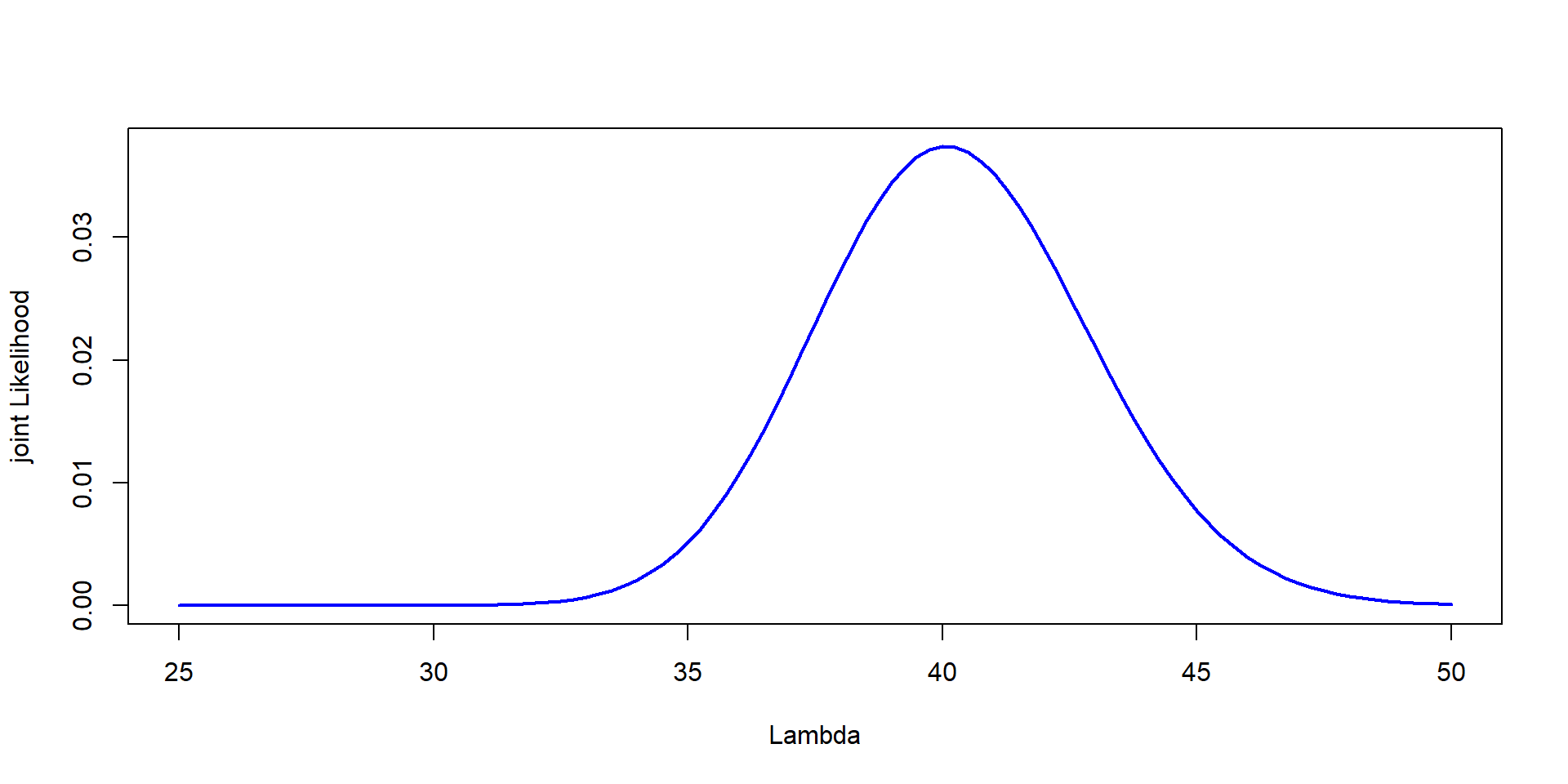
<- jointL/ sum (jointL)
Plot it
plot (Lambda,Posterior,type= "l" , col= "blue" , lwd= 2 ,ylab= "joint Likelihood" , xlab= "Lambda" )
That is the result
No point estimate. It models “uncertainty”
Median is usually reported
You can estimate 95% of the area under the curve –> credible intervals
Challenge. Bats per net
You are surveying bats near a beach. You set up one mist net and caught 8 bats
From previous surveys, you know that the mean catch per net is around 10 bats, with a standard deviation of around 3 bats
Estimate Likelihood, prior, combine them (joint) and estimate the posterior (normalized so that it sums to 1)
Plot all three on the same graph: likelihood, prior, and posterior –> Scale the prior and likelihood if necessary so they fit on the same plot
Find the most probable value of \(\lambda\)
For next class
Download JAGS