flowchart LR
  A[HEADS] --> B[HEADS]
  A --> C[TAILS]
  B --> D[HEADS]
  B --> E[TAILS]
  C --> F[HEADS]
  C --> G[TAILS]
Bayesian statistics
SNR 610
Today
Probability and Likelihood (step 1 out of 3)
Reminder
What is probability?
Certainty that an event will happen
Example:
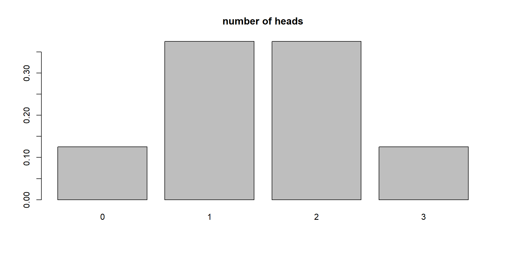
X = number of heads in 3 tosses
x = exactly 2 heads
\(\theta=0.5\) (probability)
\(P(X=x | \theta) = 3/8\)
\(P(\text{Number of heads in 3 tosses}= 2 | 0.5) = 3/8\)
Why?
flowchart LR
  A[TAILS] --> B[HEADS]
  A --> C[TAILS]
  B --> D[HEADS]
  B --> E[TAILS]
  C --> F[HEADS]
  C --> G[TAILS]
Probability
3 tosses
Probability of 1 head?
Probability of 3 heads?
Probability of 0 heads?
We treat \(\theta\) as fixed (0.5)
Probability
We can actually estimate any probability as long as we know the parameters
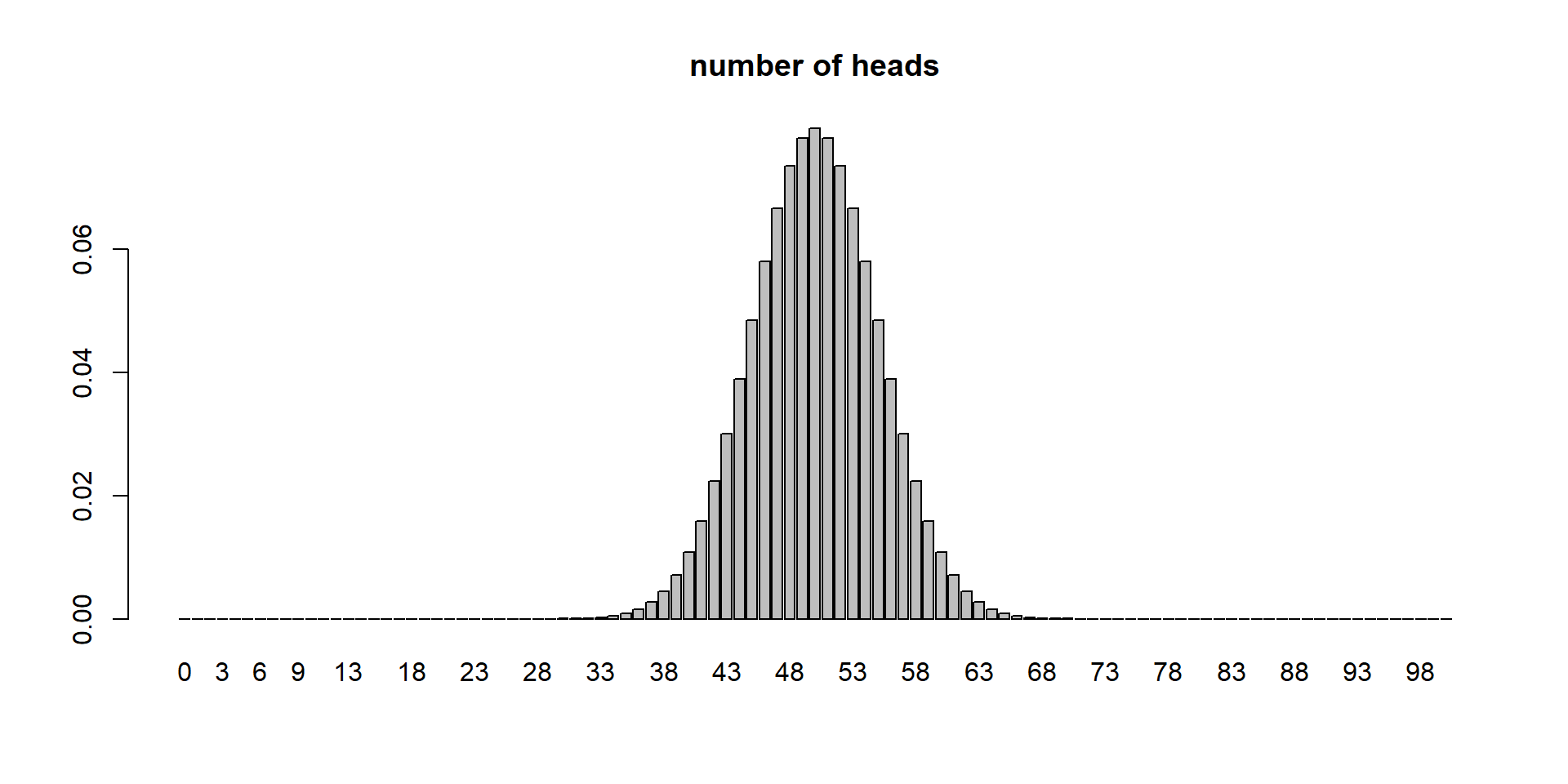
Binomial distribution parameters: n and p
n is number of trials
\(P(X=x | \theta) = Y\)
\(P(successes = x | \text{p and n}) = Y\)
\(P(successes = 12 | \text{0.5 and 50}) = 0.0001078\)
\(P(successes \ge 57 | \text{0.5 and 100}) = 0.0966\)
We use
dbinom. Like this:dbinom(x,n,p)Example:dbinom(12,50,0.5)For \(\ge\) 57:
sum(dbinom(57:n,n,p))
Probability
Probability
Probability
Parameters of binomial
Probability and n!
Parameters of a Normal distribution
Who can remember them?
Mean and sd (or variance)
For a population of males in the USA, these are the parameters:
\(\mu = 177.6cm\)
\(\sigma = 9.7cm\)
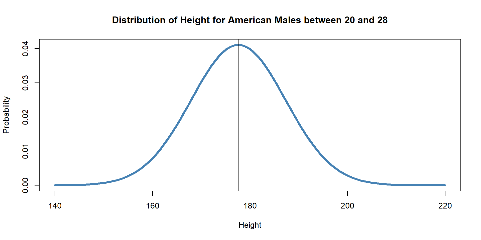
What is the probability of sampling a random man with a heigh of 172.85431 cm?
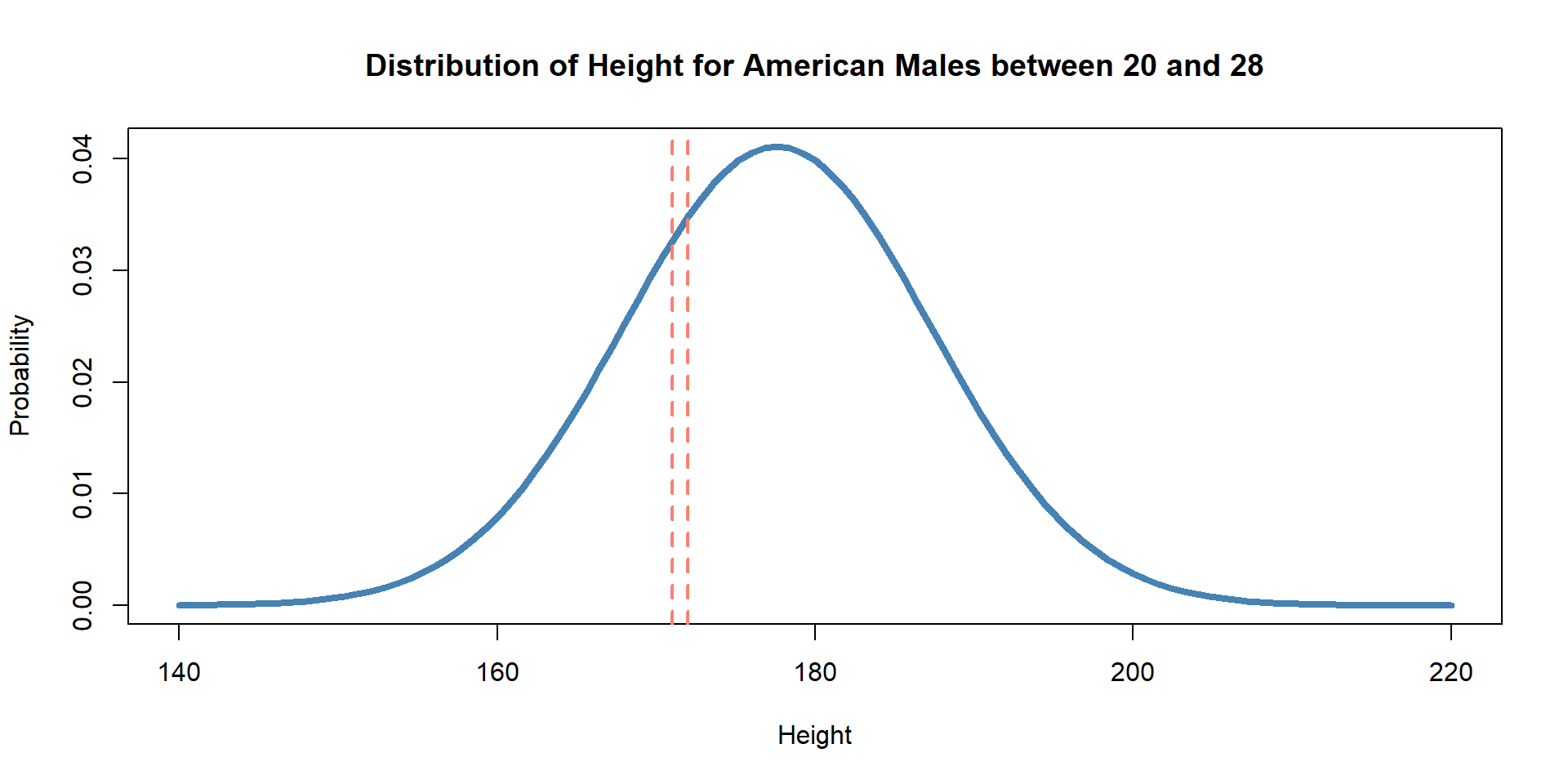
What is the probability of sampling one random man and him being between 170 and 171 cm?
Normal Distribution
By knowing the mean and sd we can plot any normal distibution
We can estimate any probability as well
Probability of observing X given the parameters
- \(P ( 170 \le X \le 171) | \mu = 177.6, \sigma = 9.7)\)
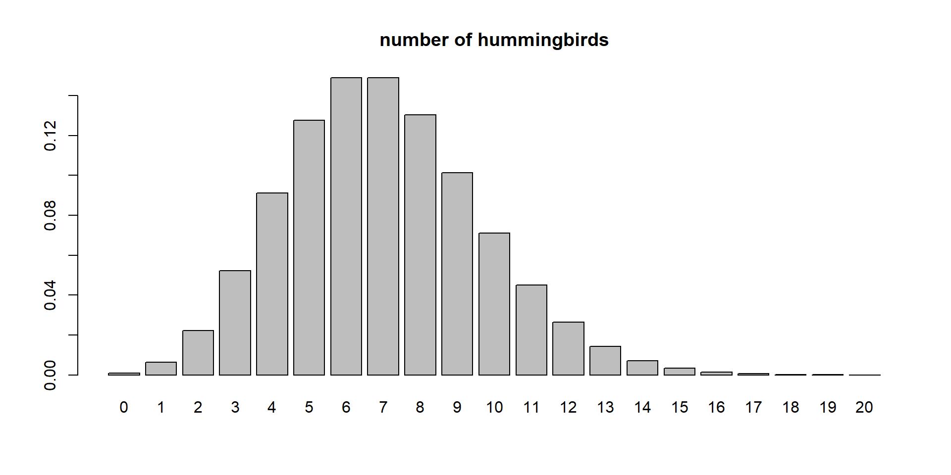
Poisson Distribution
One parameter
\(\lambda\)
Represents both mean and sd
When \(\lambda = 7\) what is the probability of seeing 5 hummingbirds visit a flower?
\(P(X=5|\lambda =7)\)
Poisson Distribution
Takeaway
Probability: Chance of an event occuring
Chance of data being something, given the parameters
The parameters do not change. For example, for a p of 0.5 we can estimate the prob of 0, 1, 2… 100 heads out of 100
Question
Test your knowledge…
- You have a coin that you do not know if it is fair or unfair. What is the probability that you will get 40 heads in 100 tosses?
Probability
We cannot estimate it if we do not have the parameters!
We usually do not have them
It is what we are trying to estimate!!!!
If we had them, there would be no point on sampling/experiments
Examples:
Probability of infection (infection rate)
Yield of a crop
Annual sales
community composition
What do we have?
Data!
Unfair or fair coin
You are smart, so you knew we couldn’t estimate it! You decide to grab the coin, and do 100 flips.
You get 65 heads and 35 tails
What value of P (prob of heads) is more likely:
0.3
0.5
0.7
We can estimate the Likelihood
Likelihood of a parameter given our data
Probability: \(P(X=x|\theta)\)
x = data and \(\theta\) = parameter
Likelihood: \(\mathcal{L}(x|\theta = y)\)
In other words
Likelihood: \(\mathcal{L}(65|p= 0.3 \; \& \; n=100)\)
Likelihood: \(\mathcal{L}(65|p= 0.5 \; \& \; n=100)\)
Likelihood: \(\mathcal{L}(65|p= 0.7 \; \& \; n=100)\)
In other words
Likelihood: \(\mathcal{L}(65|p= 0.3 \; \& \; n=100)\)
Likelihood: \(\mathcal{L}(65|p= 0.5 \; \& \; n=100)\)
Likelihood: \(\mathcal{L}(65|p= 0.7 \; \& \; n=100)\)
In other words
Likelihood: \(\mathcal{L}(65|p= 0.3 \; \& \; n=100)\)
Likelihood: \(\mathcal{L}(65|p= 0.5 \; \& \; n=100)\)
Likelihood: \(\mathcal{L}(65|p= 0.7 \; \& \; n=100)\)
In other words
Likelihood: \(\mathcal{L}(65|p= 0.3 \; \& \; n=100)\)
Likelihood: \(\mathcal{L}(65|p= 0.5 \; \& \; n=100)\)
Likelihood: \(\mathcal{L}(65|p= 0.7 \; \& \; n=100)\)
[1] 4.273205e-13[1] 0.0008638557[1] 0.04677968 [1] 7.703225e-104 1.992063e-84 3.884481e-73 3.571358e-65 4.929663e-59
[6] 4.772511e-54 7.374228e-50 2.970735e-46 4.282059e-43 2.741123e-40
[11] 9.091081e-38 1.750311e-35 2.132713e-33 1.758769e-31 1.035226e-29
[16] 4.539569e-28 1.535868e-26 4.127038e-25 9.024029e-24 1.638853e-22
[21] 2.515609e-21 3.313036e-20 3.792499e-19 3.816341e-18 3.409459e-17
[26] 2.727838e-16 1.969634e-15 1.292261e-14 7.750912e-14 4.273205e-13
[31] 2.176051e-12 1.028019e-11 4.523399e-11 1.860408e-10 7.175152e-10
[36] 2.602570e-09 8.901681e-09 2.877953e-08 8.814231e-08 2.562323e-07
[41] 7.082912e-07 1.864766e-06 4.682851e-06 1.123170e-05 2.576014e-05
[46] 5.655635e-05 1.189753e-04 2.400149e-04 4.646673e-04 8.638557e-04
[51] 1.542997e-03 2.649119e-03 4.373180e-03 6.943193e-03 1.060361e-02
[56] 1.557780e-02 2.201417e-02 2.992165e-02 3.910718e-02 4.913282e-02
[61] 5.931182e-02 6.875851e-02 7.649566e-02 8.160685e-02 8.340469e-02
[66] 8.157530e-02 7.625895e-02 6.804079e-02 5.784834e-02 4.677968e-02
[71] 3.590570e-02 2.609661e-02 1.791259e-02 1.157630e-02 7.019775e-03
[76] 3.978485e-03 2.098032e-03 1.024198e-03 4.601262e-04 1.889469e-04
[81] 7.036278e-05 2.354392e-05 7.002111e-06 1.827232e-06 4.119694e-07
[86] 7.876283e-08 1.247985e-08 1.592788e-09 1.579556e-10 1.161994e-11
[91] 5.965119e-13 1.966976e-14 3.709060e-16 3.373223e-18 1.136123e-20
[96] 9.102708e-24 7.565670e-28 1.012012e-33 5.698078e-44Likelihood
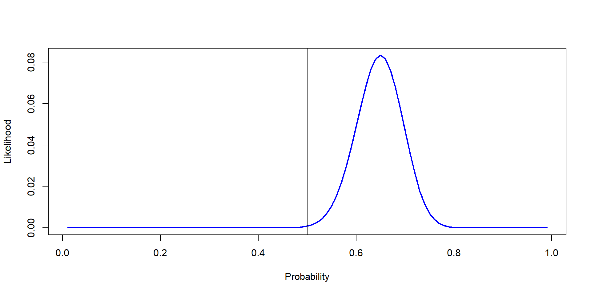
“Very Unlikely that it is fair”
Probability vs Likelihood
Probability:
Likelihood
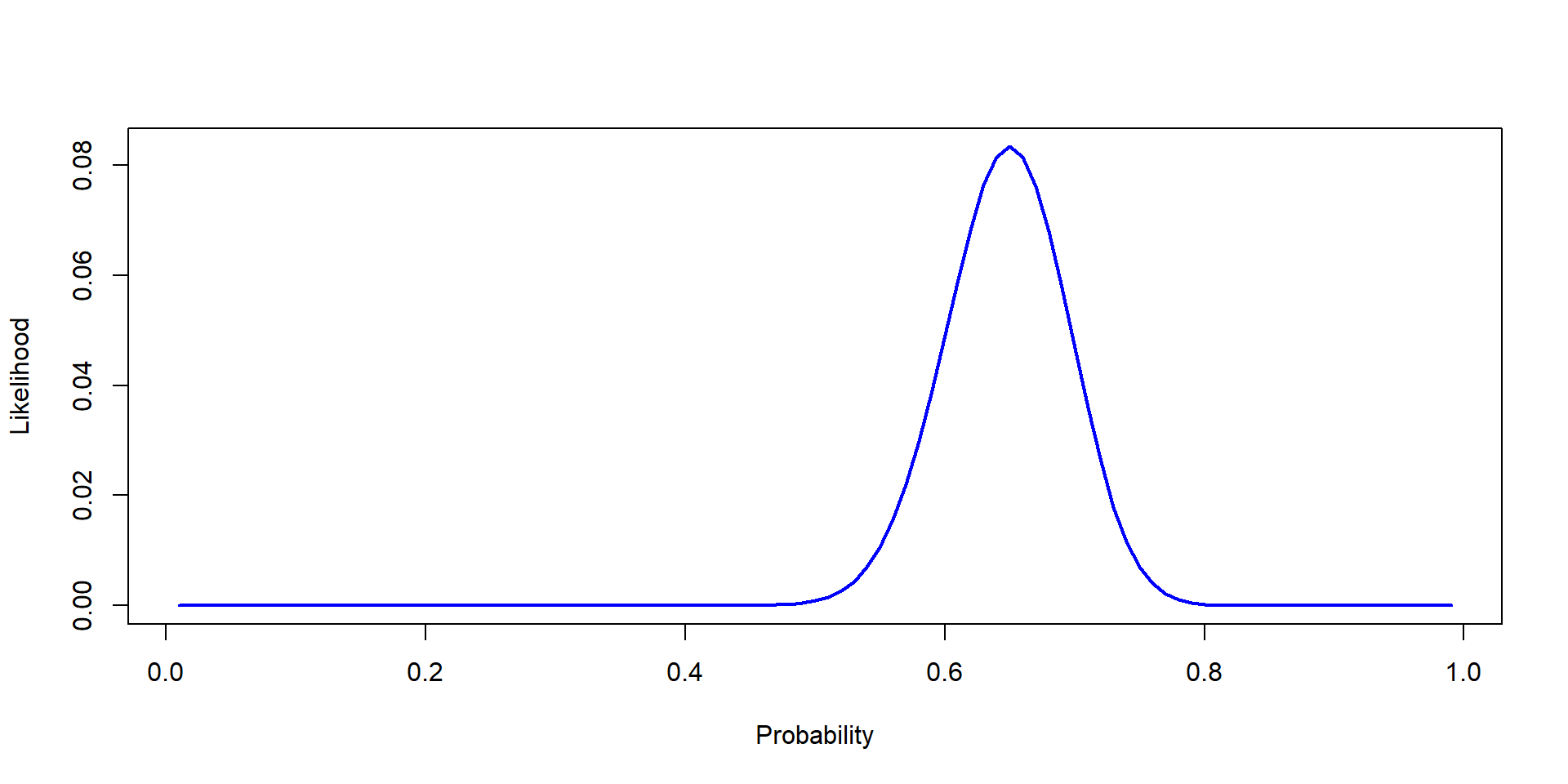
Likelihood is continuous
Review
If you capture 5 raccoons with weights of 11.2, 12, 11.5, 12.8, 11.06 is it more likely that the population mean is 11.5 or 17?
If you get 80 heads in 100 tosses, is it more likely that p is 0.8 or 0.5
If you count insects per tree and find 77, 70, 75, 86, and 90 is it more likely that \(\lambda\) for insects per tree is 60, 80, or 120?
Likelihood is estimated!
\(\mathcal{L}(x|\theta = y)\)
And usually (and correctly): \(\mathcal{L}(\theta|data)\)
We use the probability density functions
Likelihood and probability (correct way)
\[ \Huge \mathcal{L}(\theta|data) \]
\[ \Huge P(data|\theta) \]
\[ \mathcal{L}(\theta|data) = P(data|\theta) \]
- Likelihood of p being 0.5 given 48 heads out of 100 tosses
- Probability of 48 heads out of 100 tosses given a probability of 0.5
Bayesian
A different statistical framework
We have used frequentist so far
| Topic | Frequentist | Bayesian |
|---|---|---|
| Parameters | Fixed unknown | Random variable |
| Data | Random | Fixed |
| Inference | Based on a sampling distribution | Based on posterior |
| Output | P-value, Confidence intervals, betas | Credible intervals and posterior distribution |
| Computational needs | low | high |
Data, random? Yes…
\(y_i = \beta_0 + \beta_1 + \epsilon_i\)
Bayesian take away
Different way of looking at things… we will explore how
Bayes Theorem
\[ \Huge P(\theta |data) = \frac{P(data|\theta) \times P(\theta)}{P(data)} \]
- \(P(\theta|data)\) : Posterior, probability of theta, given the data
- \(P(data|\theta)\) : Likelihood! \(\mathcal{L}(\theta|data) = P(data|\theta)\)
- \(P(\theta)\): Prior (who knows what this is!)
- \(P(data)\): Marginal (who knows!)
Challenges
Challenge 1:
- You go out to a Forest that has been separated in multiple plots. You are wondering what the count of total trees per plot is (\(\lambda\)). You only can count the number of trees in one plot chosen at random. You count 37 trees, Estimate the Likelihood of different values of \(\lambda\) as well as the maximum likelihood.
Challenge 2:
- You go to the same Forest, but were able to count three plots. They had 37, 41 and 35 trees. Estimate the Likelihood of different values of \(\lambda\)