Goal: Compare tillage methods (conventional vs. no-till) and nitrogen fertilizer rates on burley tobacco yield
Design: Split-plot with tillage as the main-plot factor and fertilizer as the subplot factor
Main plots: Tillage (CT, NT) - applied to whole plots because tillage requires large equipment
Subplots: Fertilizer (0, 140, 280 kg N/ha) - can vary within a main plot
Replicates: 4 blocks (randomized complete block design at the main-plot level)
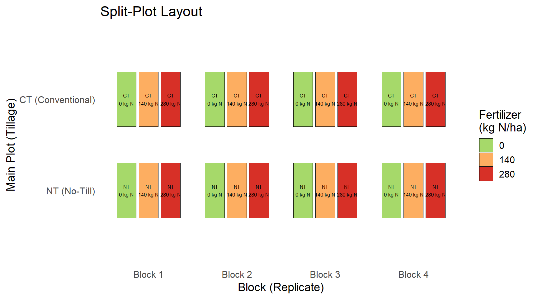
Split-Plot Design Diagram
Figure 1: Schematic of a split-plot design with 2 tillage levels and 3 fertilizer rates across 4 blocks.
Key Properties of Split-Plot Designs
Two levels of randomization:
Main-plot factor (tillage) is randomized across whole plots within each block
Subplot factor (fertilizer) is randomized within each main plot
Two error terms:
Main-plot error: variation among main plots within blocks (used to test tillage)
Subplot error: variation among subplots within main plots (used to test fertilizer and the interaction)
Why split-plot? Some factors (e.g., tillage) are hard or impractical to apply at a small scale
The Model
In R, we fit the split-plot model using lmer from the lme4 package:
# Yield ~ fixed effects + random effects# Tillage * Fertilizer = Tillage + Fertilizer + Tillage:Fertilizer# (1 | Block/WU) = random intercept for Block and whole-plot unit nested in Blockmodel <-lmer(Yield ~ Tillage * Fertilizer + (1| Block/WU), data = data)
Term
Meaning
Tillage * Fertilizer
Fixed effects: main effects and interaction
(1 | Block)
Random effect for blocks (replicates)
(1 | Block:WU)
Random effect for whole-plot units (main-plot error)
Residual
Subplot error
Fitting the Model in R
# Source the simulation and plotting code from the repo.# This script (projects/examplesplitplot.R) creates:# - data: a data.frame with Tillage, Fertilizer, Replicate, Yield, WU, Block# - model: an lmer fit (Yield ~ Tillage * Fertilizer + (1 | Block/WU))# - p: a ggplot object showing the simulated split-plot datasource("../projects/examplesplitplot.R")# Display the ANOVA tableanova(model)
Analysis of Variance Table
                   npar  Sum Sq Mean Sq  F value
Tillage               1   723.8   723.8  27.0436
Fertilizer            2 12843.6  6421.8 239.9364
Tillage:Fertilizer    2    38.1    19.1   0.7121
Model Summary
summary(model)
Linear mixed model fit by REML ['lmerMod']
Formula: Yield ~ Tillage * Fertilizer + (1 | Block/WU)
   Data: data

REML criterion at convergence: 118.6

Scaled residuals:
    Min      1Q  Median      3Q     Max
-1.7507 -0.5957 -0.0413  0.4511  1.8075

Random effects:
 Groups   Name        Variance  Std.Dev.
 WU:Block (Intercept) 0.000e+00 0.000e+00
 Block    (Intercept) 3.282e-17 5.729e-09
 Residual             2.676e+01 5.173e+00
Number of obs: 24, groups:  WU:Block, 8; Block, 4

Fixed effects:
                        Estimate Std. Error t value
(Intercept)               61.253      2.587  23.680
TillageNT                -13.575      3.658  -3.711
Fertilizer140             25.807      3.658   7.055
Fertilizer280             55.778      3.658  15.248
TillageNT:Fertilizer140    6.007      5.173   1.161
TillageNT:Fertilizer280    1.768      5.173   0.342

Correlation of Fixed Effects:
            (Intr) TllgNT Frt140 Frt280 TNT:F1
TillageNT   -0.707
Fertilzr140 -0.707  0.500
Fertilzr280 -0.707  0.500  0.500
TllgNT:F140  0.500 -0.707 -0.707 -0.354
TllgNT:F280  0.500 -0.707 -0.354 -0.707  0.500
optimizer (nloptwrap) convergence code: 0 (OK)
boundary (singular) fit: see help('isSingular')
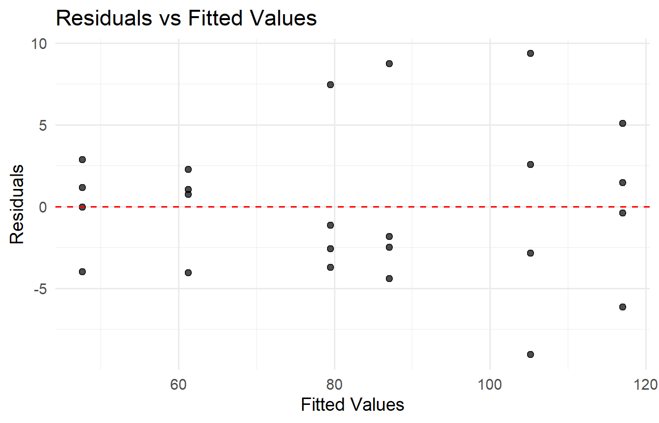
Diagnostic Plot: Residuals vs Fitted
Figure 2: Residuals vs fitted values for the split-plot model. Look for patterns indicating model misspecification.
Interpreting the Results
Main-plot effect (Tillage): Tested against the whole-plot error. A significant tillage effect means the two tillage methods produce different average yields.
Subplot effect (Fertilizer): Tested against the subplot (residual) error. A significant fertilizer effect means nitrogen rate influences yield.
Interaction (Tillage x Fertilizer): Also tested against subplot error. A significant interaction means the fertilizer effect depends on which tillage method is used.
Check: The whole-plot error variance should be non-negligible. If it is near zero, the split-plot structure may not be needed.
Practical Tips
Balance: Ensure equal replication of all treatment combinations within each block.
Blocking: Use blocks to control for known sources of variation (e.g., field position, soil type).
Diagnostics: Always check residual plots for non-constant variance or non-normality.
Random vs. fixed: The whole-plot grouping factor must be random. If you treat it as fixed, you underestimate the main-plot error.
Software:lme4::lmer and nlme::lme both handle split-plot models. Use car::Anova() or anova() for Type III tests.
Next Steps
Student activity (10 min):
Write a split-plot experiment proposal for your thesis or research area.
Identify your main-plot factor and subplot factor.
Describe how you would analyze the data (e.g., write out the lmer call).