Matching Methods to Research Questions
The Method-Question-Data Triangle
2001-03-01
The Problem
We often learn methods in isolation –> during classes
- “This is a t-test”
- “This is ANOVA”
- “This is regression”
- “This is Bayesian”
Then we want to apply those methods in our data.
This is particularly true for people that really enjoy analytical methods!
This is backwards!
The research question should drive everything!
The Triangle Framework
         RESEARCH QUESTION
                /\
               /  \
              /    \
             /      \
            /        \
           /          \
    DATA TYPE -------- METHOD CHOICE
All three must align
Misalignment leads to:
- Wrong conclusions
- Wasted effort
- Rejected papers
- Sad grad students! 😦
Research Question Drives Everything
| Question Type | What You’re Looking For | Example Methods |
|---|---|---|
| Is there a difference? | Comparison | t-test, ANOVA, GLM |
| Is there a relationship? | Association | Regression, correlation |
| Can I predict? | Prediction | ML, regression |
| What’s the pattern? | Structure | Clustering, PCA, ordination |
Your question determines what “answer” looks like!
Data Type Constrains Your Options
| Response Variable | Distribution | Common Methods |
|---|---|---|
| Continuous, normal | Gaussian | LM, ANOVA |
| Counts (0, 1, 2, …) | Poisson, NegBin | GLM |
| Binary (yes/no) | Binomial | Logistic regression |
| Proportions (0-1) | Binomial, Beta | GLM, Beta regression |
Also consider:
- Independence vs. grouping
- Repeated measures
- Nested/hierarchical structure
The Alignment Check ✅
Before analyzing, ask yourself:
✅ What exactly is my question?
✅ What type of response variable do I have?
✅ What is my data structure (grouping, nesting, time)?
✅ Does my method handle all of this?
If you can’t answer these → STOP and think!
Three Common Scenarios
We’ll look at three examples:
Mismatch - Method ignores key data structure
Good Match - Method fits question and data
Overcomplicated - Method is fancier than needed
Let’s see each one…
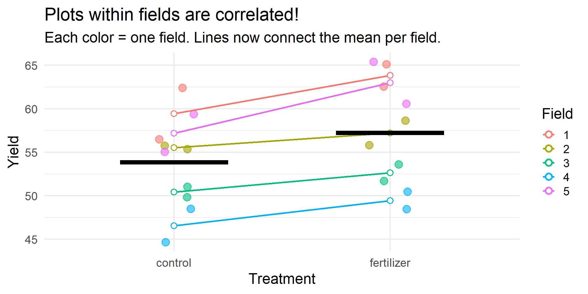
Example 1: MISMATCH
Scenario:
- Testing fertilizer effect on crop yield
- 5 fields, 4 plots per field
- 2 control plots, 2 fertilized plots per field
Example 1: The Problem
Example 1: Wrong vs. Right
TRUE EFFECT: 3 unitsWRONG MODEL (lm): Estimate: 3.38 Std Error: 2.57 p-value: 0.2043 CORRECT MODEL (lmer): Estimate: 3.38 Std Error: 0.99 p-value: 0 Example 1: The Fix
In this design (treatment within fields):
- The wrong model has inflated standard errors because it treats field variance as residual noise
- The correct model* separates field variance → cleaner estimate of treatment effect
- This means reduced power when you ignore structure
In other designs (treatment between fields):
- Ignoring structure would inflate Type I error instead
Lesson: Always check your independence assumption!
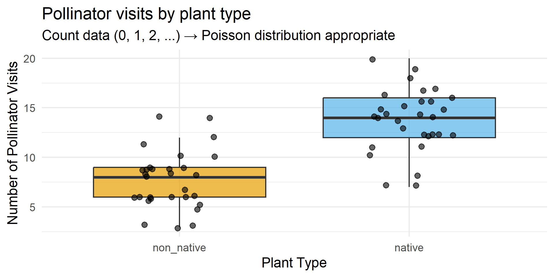
Example 2: GOOD MATCH
Scenario:
- Pollinator visits to flowers
- 2 treatments: native vs. non-native plants
- 30 plants per treatment
- Response: count of visits (0 to ~45)
Example 2: The Data
Example 2: Why It Works
Show code
                 Estimate Std. Error   z value      Pr(>|z|)
(Intercept)     2.0412203  0.0657951 31.023896 2.567154e-211
treatmentnative 0.5761755  0.0822319  7.006715  2.439777e-12
Checklist:
- ✅ Count data → Poisson distribution
- ✅ No upper bound on counts
- ✅ Independent observations (different plants)
- ✅ Simple comparison question
Example 2: Interpretation
Show code
Coefficient (log scale): 0.576 Multiplicative effect: 1.78 Native plants get 77.9 % more visitsLesson: Match your distribution to your data type!
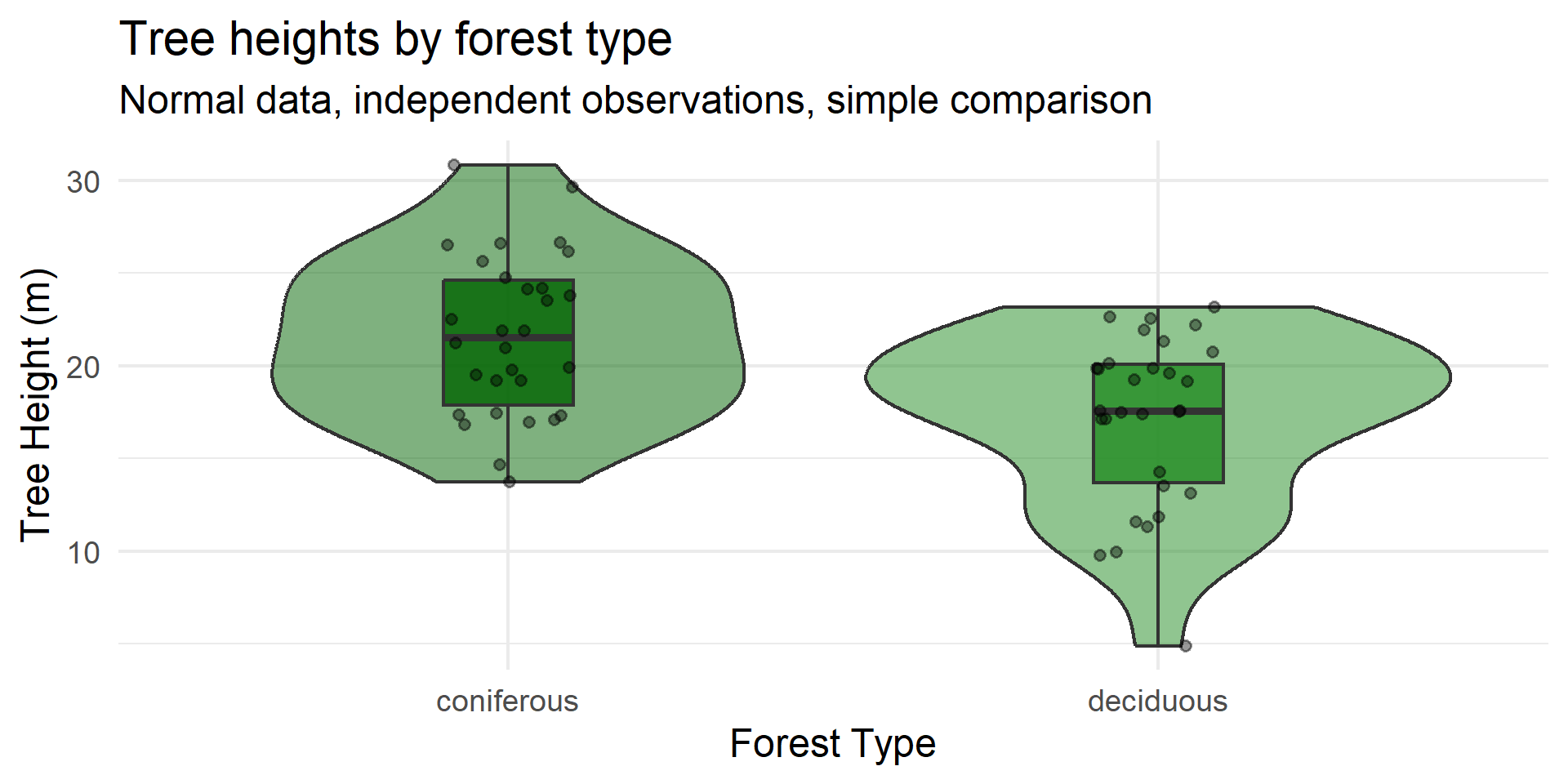
Example 3: OVERCOMPLICATED
Scenario:
- Tree height in 2 forest types
- 30 trees per forest type
- Normal distribution, no grouping
- Simple question: “Is there a difference?”
The overkill:
“Let’s use a Bayesian hierarchical model with spatial autocorrelation, weakly informative priors, and MCMC sampling!”
Example 3: The Data
Example 3: Simple vs. Complex
Show code
Difference: -4.51 metersShow code
95% CI: [ 2.2 , 6.81 ]p-value: 0.000239 Time to run: ~0.001 seconds
A Bayesian spatial model: ~5-10 minutes
Same answer!
Example 3: The Lesson
Problems with overcomplication:
- Takes much longer to fit
- Harder to interpret
- Reviewers get confused
- More things can go wrong
- Same answer as simple approach!
Principle of parsimony:
Use the simplest method that adequately addresses your question
Save fancy methods for when you need them!
I know this is challenging! When I learn about new methods, I want to use them ALL THE TIME. But resist the urge! Focus on the researhc question!
If you teach, you get to explore any methods you want in your lessons!
Summary: Three Scenarios
| Example | Problem | Consequence | Lesson |
|---|---|---|---|
| Mismatch | Ignored grouping structure | False positive risk | Check independence |
| Good Match | None - appropriate method | Valid inference | Match distribution |
| Overcomplicated | Unnecessary complexity | Wasted effort | Start simple |
Your Checklist
Before you analyze, ask:
1️⃣ What is my question? (difference, relationship, prediction)
2️⃣ What is my response variable? (continuous, count, binary, proportion)
3️⃣ What is my data structure? (independent, grouped, nested, repeated)
4️⃣ Does my method handle all three?
The Golden Rule
Start simple.
. . .
Add complexity only when needed.
. . .
Always justify your choices.
Now It’s Your Turn!
Think-Pair-Share (5 min)
Look back at your silent reflection sheet. Based on the three examples:
- What method might be appropriate for YOUR data?
- What’s one thing about your data structure that makes method choice tricky?
- Think (<1 min) — you already did this… you can use 30 seconds to update your notes
- Pair (3 min) — discuss with a neighbor, help each other troubleshoot
- Share (1 min) — 2–3 volunteers share their pairing’s most interesting dilemma
Grab your worksheet and let’s go!
Now It’s Your Turn!
Data Detective Stations
- 6 scenarios around the room
- Diagnose: Mismatch? Good match? Overcomplicated?
- Work in pairs
- 4 minutes per station
Grab your worksheet and let’s go!
Appendix: Full Simulation Code
Show code
# ============================================================================
# EXAMPLE 1: MISMATCH - Ignoring nested structure
# Demonstrates FALSE POSITIVE from pseudoreplication
# ============================================================================

library(lme4)
library(ggplot2)
library(dplyr)

set.seed(42)

n_fields <- 5
n_plots_per_field <- 4

mismatch_data <- expand.grid(
  field = factor(1:n_fields),
  plot = 1:n_plots_per_field
) |>
  mutate(
    treatment = rep(c("control", "control", "fertilizer", "fertilizer"), n_fields),
    treatment = factor(treatment, levels = c("control", "fertilizer"))
  )

# Large field-to-field variation
field_effects <- data.frame(
  field = factor(1:n_fields),
  field_effect = c(-12, -5, 2, 8, 14)
)

true_effect <- 0  # NO TRUE EFFECT!

mismatch_data <- mismatch_data |>
  left_join(field_effects, by = "field") |>
  mutate(
    yield = 50 + field_effect +
            ifelse(treatment == "fertilizer", true_effect, 0) +
            rnorm(n(), mean = 0, sd = 1.5)
  ) |>
  # Create confounding between treatment and field quality
  mutate(
    yield = yield + ifelse(treatment == "fertilizer", field_effect * 0.15, 0)
  )

# Compare wrong vs correct
wrong_model <- lm(yield ~ treatment, data = mismatch_data)
correct_model <- lmer(yield ~ treatment + (1|field), data = mismatch_data)

# Wrong model shows "significant" effect (p < 0.05)
summary(wrong_model)

# Correct model shows non-significant (as it should be - no true effect!)
summary(correct_model)
Appendix: Full Simulation Code (continued)
Show code
# ============================================================================
# EXAMPLE 2: GOOD MATCH - Poisson GLM for counts
# ============================================================================

set.seed(2024)
n_per_group <- 30

goodmatch_data <- data.frame(
  plant_id = 1:(2 * n_per_group),
  treatment = factor(rep(c("native", "non_native"), each = n_per_group),
                     levels = c("non_native", "native"))
)

baseline_visits <- 8
native_effect <- 0.5  # Log-scale

goodmatch_data <- goodmatch_data |>
  mutate(
    log_mu = log(baseline_visits) +
             ifelse(treatment == "native", native_effect, 0),
    visits = rpois(n(), lambda = exp(log_mu))
  )

poisson_model <- glm(visits ~ treatment, family = poisson,
                     data = goodmatch_data)
summary(poisson_model)

# Interpretation
exp(coef(poisson_model)["treatmentnative"])  # Multiplicative effect
Appendix: Full Simulation Code (continued)
Show code
# ============================================================================
# EXAMPLE 3: OVERCOMPLICATED - Simple question, complex method
# ============================================================================

set.seed(2024)
n_trees <- 30

overcomp_data <- data.frame(
  tree_id = 1:(2 * n_trees),
  forest_type = factor(rep(c("deciduous", "coniferous"), each = n_trees))
)

deciduous_mean <- 18
coniferous_mean <- 22
tree_sd <- 4

overcomp_data <- overcomp_data |>
  mutate(
    height = ifelse(forest_type == "deciduous",
                    rnorm(n(), deciduous_mean, tree_sd),
                    rnorm(n(), coniferous_mean, tree_sd))
  )

# Simple and appropriate!
t.test(height ~ forest_type, data = overcomp_data)

# Or equivalently
lm(height ~ forest_type, data = overcomp_data) |> summary()